Skip to content
Free Excel Tutorials
  • Home
  • Excel For Beginners
  • Excel Intermediate
  • Advanced Excel For Experts

Data Analysis

  • Conditional Formatting Icon Sets Examples in Excel
  • Example of COUNTIFS with variable table column in Excel
  • How to Use Solver Tool in Excel
  • What-If Analysis: Scenarios and Goal Seek in Excel
  • Create Scatter Chart in Excel

References

  • Vlookup Examples in Excel
  • How to get last column number in range in Excel
  • INDEX function: Description, Usage, Syntax, Examples and Explanation
  • Basic INDEX MATCH approximate in Excel
  • VLOOKUP function: Description, Usage, Syntax, Examples and Explanation

Data Validations

  • Excel Data validation allow uppercase only
  • Excel Data validation with conditional list
  • Data validation must not exist in list
  • Excel Data validation number multiple 100
  • Excel Data validation must begin with

Get position of 2nd 3rd and more instance of character in Excel

by

To get the position of the 2nd, 3rd, 4th, etc. instance of a specific character inside a text string, you can use the FIND and SUBSTITUTE functions.

Note: we use “~” in this case only because it rarely occurs in other text. You can use any character that you know won’t appear in the text.

Formula

=FIND("~",SUBSTITUTE(text,char,"~",instance))

Explanation

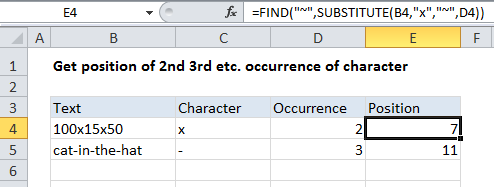
In the example shown, the formula in E4 is:

=FIND("~",SUBSTITUTE(B4,"x","~",D4))

How this formula works

At the core, this formula uses the fact that the SUBSTITUTE function understands “instance”, supplied as an optional forth argument called “instance_num”. This means you can use the SUBSTITUTE function to replace a specific instance of a character in a text string.  So:

SUBSTITUTE(B4,"x","~",D4)

replaces only the 2nd instance (2 comes from D4) of “x” in text in B4, with “~” character. The result looks like this:

100×15~50

Next, FIND locates the “~” inside this string and returns the position, which is 7 in this case.

Post navigation

Next Post:

Create One-dimensional and Two-dimensional Array

Leave a Reply Cancel reply

Your email address will not be published. Required fields are marked *

Learn Basic Excel

Ribbon
Workbook
Worksheets
Format Cells
Find & Select
Sort & Filter
Templates
Print
Share
Protect
Keyboard Shortcuts

Categories

  • Charts
  • Data Analysis
  • Data Validation
  • Excel Functions
    • Cube Functions
    • Database Functions
    • Date and Time Functions
    • Engineering Functions
    • Financial Functions
    • Information Functions
    • Logical Functions
    • Lookup and Reference Functions
    • Math and Trig Functions
    • Statistical Functions
    • Text Functions
    • Web Functions
  • Excel VBA
  • Excel Video Tutorials
  • Formatting
  • Grouping
  • Others

Logical Functions

  • How to return blank in place of #DIV/0! error in Excel
  • IF, AND, OR and NOT Functions Examples in Excel
  • IFERROR function: Description, Usage, Syntax, Examples and Explanation
  • How to use Excel FALSE Function
  • How to use IFS function in Excel

Date Time

  • Calculate date overlap in days in Excel
  • Get last working day in month in Excel
  • Check If Two Dates are same month in Excel
  • DATEDIF function: Description, Usage, Syntax, Examples and Explanation
  • Calculate total hours that fall between two times in Excel

Grouping

  • Map inputs to arbitrary values in Excel
  • Calculate conditional mode with criteria in Excel
  • Group arbitrary text values in Excel
  • Group numbers with VLOOKUP in Excel
  • Group times into unequal buckets in Excel

General

  • Count cells less than in Excel
  • How to fill cell ranges with random number from fixed set of options in Excel
  • List sheet names with formula in Excel
  • How to fill cell ranges with random text values in Excel
  • Index and match on multiple columns in Excel
© 2026 xlsoffice . All Right Reserved. | Teal Smiles | Abbreviations And Their Meaning