
Skip to content
Free Excel Tutorials
  • Home
  • Excel For Beginners
  • Excel Intermediate
  • Advanced Excel For Experts

Data Analysis

  • Conditional Formatting Data bars Examples in Excel
  • How to Create Gantt Chart in Excel
  • How To Compare Two Lists in Excel
  • Excel Bar Chart
  • How To Remove Duplicates In Excel Column Or Row?

References

  • Offset in Excel
  • How to get last column number in range in Excel
  • Create hyperlink with VLOOKUP in Excel
  • Count rows with at least n matching values
  • Two-way lookup with VLOOKUP in Excel

Data Validations

  • Excel Data validation exists in list
  • Excel Data validation unique values only
  • Excel Data validation date in specific year
  • How To Create Drop-down List in Excel
  • Excel Data validation number multiple 100

Excel Rank without ties Example

by

This tutorials shows how to Rank numbers without  ties  in Excel.

To assign rank without ties, you can use a formula based on the RANK and COUNTIF functions.

Formula

=RANK(A1,range)+COUNTIF(exp_range,A1)-1
Explanation

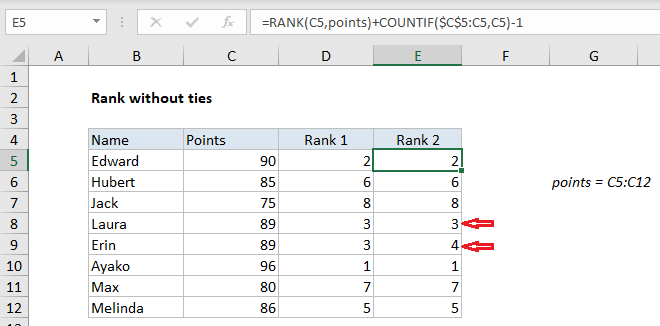
In the example shown, the formula in E5 is:

=RANK(C5,points)+COUNTIF($C$5:C5,C5)-1

where “points” is the named range

How this formula works

This formula breaks ties with a simple approach: this first tie in a list “wins” and is assigned the higher rank. The first part of the formula uses the RANK function normally:

=RANK(C5,points)

Rank returns a computed rank, which will include ties when the values being ranked include duplicates. Note the the RANK function by itself will assign the same rank to duplicate values, and skip the next rank value. You can see this in the Rank 1 column, rows 8 and 9 in the worksheet.

The second part of the formula breaks the tie with COUNTIF:

COUNTIF($C$5:C5,C5)-1

Note the range we give COUNTIF is an expanding reference: the first reference is absolute and the second is relative. As long as a value appears just once, this expression cancels itself out – COUNTIF returns 1, from which 1 is subtracted.

However, when a duplicate number is encountered, COUNTIF returns 2, the expression returns 1, and the rank value is increased by 1. Essentially, this “replaces” the rank value that was skipped originally.

The same process repeats as the formula is copied down the column. If another duplicate is encountered, the rank value is increased by 2, and so on.

Post navigation

Previous Post:

DECIMAL function: Description, Usage, Syntax, Examples and Explanation

Next Post:

AVERAGE function: Description, Usage, Syntax, Examples and Explanation

Leave a Reply Cancel reply

Your email address will not be published. Required fields are marked *

Learn Basic Excel

Ribbon
Workbook
Worksheets
Format Cells
Find & Select
Sort & Filter
Templates
Print
Share
Protect
Keyboard Shortcuts

Categories

  • Charts
  • Data Analysis
  • Data Validation
  • Excel Functions
    • Cube Functions
    • Database Functions
    • Date and Time Functions
    • Engineering Functions
    • Financial Functions
    • Information Functions
    • Logical Functions
    • Lookup and Reference Functions
    • Math and Trig Functions
    • Statistical Functions
    • Text Functions
    • Web Functions
  • Excel VBA
  • Excel Video Tutorials
  • Formatting
  • Grouping
  • Others

Logical Functions

  • How to use Excel NOT Function
  • How to return blank in place of #DIV/0! error in Excel
  • OR function Examples in Excel
  • Extract multiple matches into separate rows in Excel
  • How to use Excel XOR Function

Date Time

  • Pad week numbers with zeros in Excel
  • Count holidays between two dates in Excel
  • Sum race time splits in Excel
  • Get work hours between dates in Excel
  • Get days, months, and years between dates in Excel

Grouping

  • Calculate conditional mode with criteria in Excel
  • Map inputs to arbitrary values in Excel
  • How to randomly assign data to groups in Excel
  • Group arbitrary text values in Excel
  • Group numbers at uneven intervals in Excel

General

  • Currency vs Accounting Format in Excel
  • Find, Trace and Correct Errors in Excel Formulas using ‘Formula Auditing’
  • Cell References: Relative, Absolute and Mixed Referencing Examples
  • How to calculate percent of students absent in Excel
  • How to Insert Cells, Row and Rows in Excel
© 2026 xlsoffice . All Right Reserved. | Teal Smiles | Abbreviations And Their Meaning