Skip to content
Free Excel Tutorials
  • Home
  • Excel For Beginners
  • Excel Intermediate
  • Advanced Excel For Experts

Data Analysis

  • How to Create Area Chart in Excel
  • How to create a Histogram in Excel
  • Conflicting Multiple Conditional Formatting Rules in Excel
  • How to Use Solver Tool in Excel
  • Conditional Formatting Icon Sets Examples in Excel

References

  • How to reference named range different sheet in Excel
  • How to get relative row numbers in a range in Excel
  • Extract data with helper column in Excel
  • INDEX function: Description, Usage, Syntax, Examples and Explanation
  • Get nth match with INDEX / MATCH in Excel

Data Validations

  • Excel Data validation unique values only
  • Excel Data validation no punctuation
  • Excel Data validation with conditional list
  • How To Create Drop-down List in Excel
  • Prevent invalid data entering in specific cells

Sum visible rows in a filtered list in Excel

by

This tutorial shows how to Sum visible rows in a filtered list in Excel using the example below;

Formula

=SUBTOTAL(9,range)

Explanation

If you want to sum only the visible rows in a filtered list (i.e. only those rows not filtered out), you can use the SUBTOTAL function with function number 9 or 109. What makes SUBTOTAL especially useful is that it automatically ignores rows that are hidden in a filtered list or table.

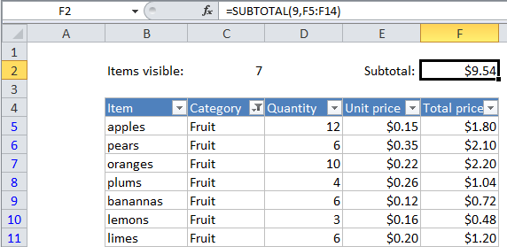
Following the example in the screen above, to sum cells in column F for visible rows only, use:

=SUBTOTAL(9,F5:F14)

If you are hiding rows manually (i.e. right-click, Hide), use this version instead:

=SUBTOTAL(109,F5:F14)

By changing the function number, the SUBTOTAL function can perform many other calculations (e.g. COUNT, SUM, MAX, MIN, etc.).

Post navigation

Previous Post:

How to use Excel CHOOSE Function

Next Post:

Customize Ribbon In Excel

Leave a Reply Cancel reply

Your email address will not be published. Required fields are marked *

Learn Basic Excel

Ribbon
Workbook
Worksheets
Format Cells
Find & Select
Sort & Filter
Templates
Print
Share
Protect
Keyboard Shortcuts

Categories

  • Charts
  • Data Analysis
  • Data Validation
  • Excel Functions
    • Cube Functions
    • Database Functions
    • Date and Time Functions
    • Engineering Functions
    • Financial Functions
    • Information Functions
    • Logical Functions
    • Lookup and Reference Functions
    • Math and Trig Functions
    • Statistical Functions
    • Text Functions
    • Web Functions
  • Excel VBA
  • Excel Video Tutorials
  • Formatting
  • Grouping
  • Others

Logical Functions

  • IF with boolean logic in Excel
  • XOR function: Description, Usage, Syntax, Examples and Explanation
  • How to use Excel NOT Function
  • Nested IF function example in Excel
  • How to return blank in place of #DIV/0! error in Excel

Date Time

  • Convert decimal hours to Excel time
  • YEAR function: Description, Usage, Syntax, Examples and Explanation
  • Basic Overtime Calculation Formula in Excel
  • Calculate time difference in hours as decimal value in Excel
  • Generate series of dates by weekends in Excel

Grouping

  • Map text to numbers in Excel
  • Group numbers at uneven intervals in Excel
  • Categorize text with keywords in Excel
  • If cell contains one of many things in Excel
  • Group arbitrary text values in Excel

General

  • Zoom Worksheet in Excel
  • Index and match on multiple columns in Excel
  • Transpose: Switch ‘Rows to Columns’ or ‘Columns to Rows’ in Excel
  • Cell References: Relative, Absolute and Mixed Referencing Examples
  • How to calculate percent of goal in Excel
© 2025 xlsoffice . All Right Reserved. | Teal Smiles | Abbreviations And Their Meaning