How to test a range for numbers in Excel

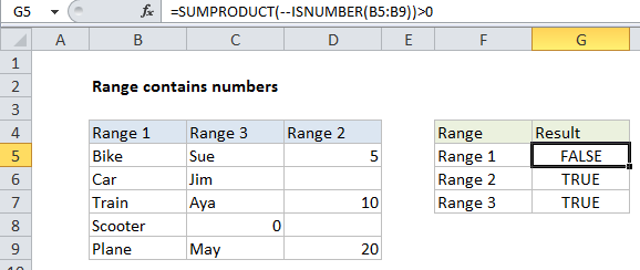
In the example shown, the formula in xxxx is:

=SUMPRODUCT(--ISNUMBER(C5:C9))>0

How this formula works

Working from the inside out, the ISNUMBER function will return TRUE when given a number and FALSE if not.

When you supply a range of references to ISNUMBER (i.e. an array), ISNUMBER will return an array of results. In the example, this array looks like this:

{FALSE;FALSE;FALSE;TRUE;FALSE}

We want to know if this result contains any TRUE values, and the easiest way to check this is to force the TRUE FALSE values to ones and zeros, then add up the result.

The double negative operator (–) will force the TRUE and FALSE values to 1 and 0 respectively, yielding an array like this:

{0;0;0;1;0}

SUMPRODUCT then adds up the items in the array and returns the result.

Any result greater than zero means that at least one number exists in the range, so we we use “>0” to evaluate and return TRUE or FALSE.