How to create simple in-cell histogram in Excel

To create a simple in-cell histogram, you can use a formula based on the REPT function. This can be handy when you have straightforward data, and want to avoid the complexity of a separate chart.

Formula

=REPT(barchar,value/100)

Explanation

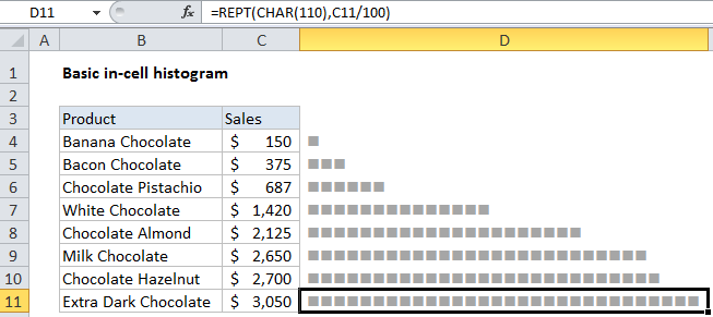
In the example shown, the formula is:

=REPT(CHAR(110),C11/100)

How this formula works

The REPT function simply repeats values. For example, this formula outputs 10 asterisks:

=REPT("*",10) // outputs **********

You can use REPT to repeat any character(s) you like. In this example, we use the CHAR function to output a character with a code of 110. This character, when formatted with the Wingdings font, will output a solid square.

CHAR(110) // square in Wingdings

To calculate the “number of times” for REPT, we scale values in column C by dividing each value by 100.

C11/100 // scale values down

This has the effect of outputting one full square per 100 dollars of sales. Increase or decrease the divisor to suit the data and available space.

Alternatively, Conditional formatting can be used

You can also use the “data bars” feature in conditional formatting to display an in cell bar.