Forecast vs Trend Function in Excel

The FORECAST and TREND function give the exact same result.

When you add a trendline to an Excel chart, Excel can display the equation in a chart (see below). You can use this equation to calculate future sales.

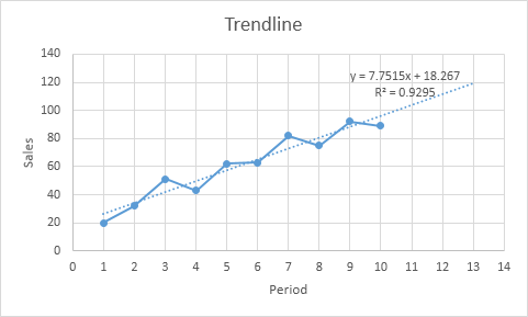
Explanation: Excel uses the method of least squares to find a line that best fits the points. The R-squared value equals 0.9295, which is a good fit. The closer to 1, the better the line fits the data.

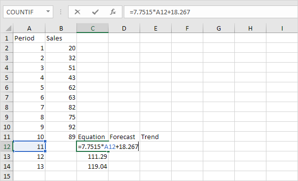
1. Use the equation to calculate future sales.

2. Use the FORECAST function to calculate future sales.

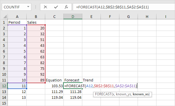
Note: when we drag the FORECAST function down, the absolute references ($B$2:$B$11 and $A$2:$A$11) stay the same, while the relative reference (A12) changes to A13 and A14.

3. If you prefer to use an array formula, use the TREND function to calculate future sales.

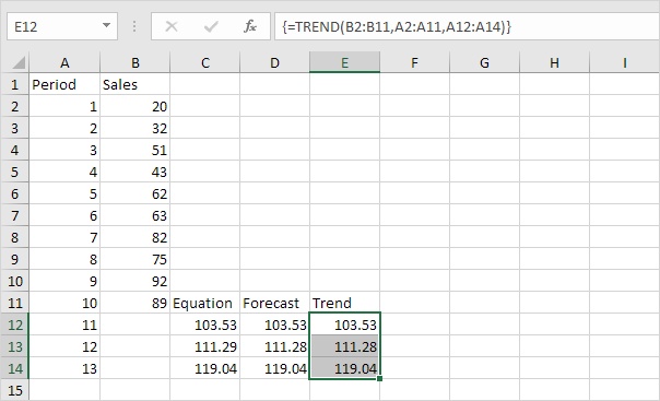
Note: first, select the range E12:E14. Next, type =TREND(B2:B11,A2:A11,A12:A14). Finish by pressing CTRL + SHIFT + ENTER. The formula bar indicates that this is an array formula by enclosing it in curly braces {}. To delete this array formula, select the range E12:E14 and press Delete.