Highlight row and column intersection exact match in Excel

This tutorial shows how to Highlight row and column intersection exact match in Excel using the example below;

Formula

=OR($A1=row_val,A$1=col_val)

Explanation

To highlight intersecting row(s) and column(s) with conditional formatting based on exact matching, you can use a simple formula based on mixed references and the OR function.

In the example shown, the formula used to apply conditional formatting is:

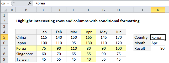
=OR($B4=$K$5,B$4=$K$6)

How this formula works

Conditional formatting is evaluated relative to every cell it is applied to, starting with the active cell in the selection, cell B3 in this case.

To highlight matching rows, we use this logical expression:

$B4=$K$5

The reference to B4 is mixed, with the column locked and row unlocked, so that only values in column B are compared to the country in cell K5. The reference to K5 is absolute, to prevent changes when the conditional formatting is applied to every cell in the range B4:H9. In the example shown, this logical expression will return TRUE for every cell in a row where country is “Korea”.

To highlight matching columns, we use this logical expression:

B$4=$K$6

The reference to B4 is again mixed. This time, the row is locked and the column is relative, so that only values in row 4 are compared to the month value in cell K6. The reference to K6 is absolute, so that it won’t change when the conditional formatting is applied to every cell B4:H9. In the example shown, this logical expression will return TRUE for every cell in a column where row 3 is “Apr”.

Because we are triggering the same conditional formatting (light yellow fill) for both rows and columns, we wrap the logical expressions above in the OR function. When either (or both) logicals return TRUE, the rule is triggered and the formatting is applied.

Highlight intersection only

To highlight the intersection only, just replace the OR function with the AND function:

=AND($B4=$K$5,B$4=$K$6)