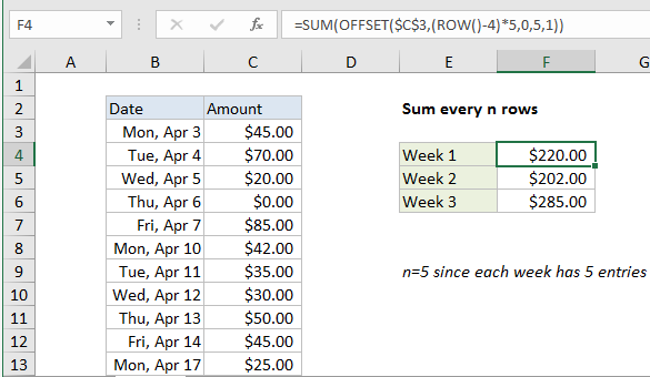
Sum every n rows in Excel

This tutorial shows how to Sum every n rows in Excel using the example below;

Formula

=SUM(OFFSET(A1,(ROW()-offset)*n,0,n,1))

Explanation

To sum every n rows, you can use a formula based on the OFFSET and SUM functions. In the example show, the formula in F4 is:

=SUM(OFFSET($C$3,(ROW()-4)*5,0,5,1))

How this formula works

In this example, there are 5 rows of data for each week (Mon-Fri) so we want to sum every 5 rows. To build a range that corresponds to the right 5 rows in each week, we use the OFFSET function. In F4 we have:

OFFSET($C$3,(ROW()-4)*5,0,5,1)

Cell C3 is the reference, entered as an absolute reference. The next argument is row, the crux of the problem. We need logic that will figure out the correct starting row for each week. For this, we use the ROW function. Because the formula sits in row 4, ROW() will return 4. We use this fact to create the logic we need, subtracting 4, and multiplying the result by 5:

(ROW()-4)*5

This will generate a row argument of 0 in F4, 5 in F5, and 10 in F6.

Column is input as zero, height as 5, and width as 1.

The OFFSET function then returns a range to SUM (the range C3:C7 for F4), and SUM returns the sum of all amounts in that range.