Skip to content
Free Excel Tutorials
  • Home
  • Excel For Beginners
  • Excel Intermediate
  • Advanced Excel For Experts

Data Analysis

  • How to create running total in an Excel Table
  • How to add Trendline to a chart in Excel
  • Use Data Form to input, edit and delete records in Excel
  • Number and Text Filters Examples in Excel
  • Conflicting Multiple Conditional Formatting Rules in Excel

References

  • How to get address of first cell in range in Excel
  • Convert text string to valid reference in Excel using Indirect function
  • How to get last row in mixed data with blanks in Excel
  • Get nth match with INDEX / MATCH in Excel
  • How to calculate two-way lookup VLOOKUP in Excel Table

Data Validations

  • Excel Data validation with conditional list
  • Excel Data validation whole percentage only
  • Excel Data validation specific characters only
  • Prevent invalid data entering in specific cells
  • Excel Data validation must not contain

Count cells not equal to x or y in Excel

by

This tutorial shows how to Count cells not equal to x or y in Excel using the example below;

Formula

=COUNTIFS(range,"<>x",range,"<>y")

Explanation

To count cells not equal to this or that, you can use the COUNTIFS function with multiple criteria.

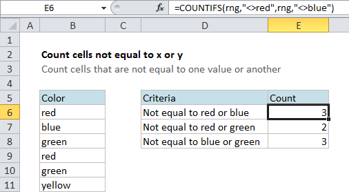
In the example shown, there is a simple list of colors in column B. There are 6 cells total with a color, and a few are duplicates.

To count the number of cells that are not equal to “red” or “blue”, the formula in E6 is:

=COUNTIFS(rng,"<>red",rng,"<>blue")

In this example “rng” is a named range that equals B6:B11.

How this formula works

The COUNTIFS function counts cells that meet one or more conditions. All conditions must pass in order for a cell to be counted.

The key in this case is to use the “not equals” operator, which is <>.

To add another criteria, simply add a another range / criteria pair of arguments.

Alternative with SUMPRODUCT

The SUMPRODUCT function can also count cells that meet multiple conditions.

For the above example, the syntax for SUMPRODUCT is:

=SUMPRODUCT((range<>"blue")*(range<>"green"))

Post navigation

Previous Post:

How to use Excel CHOOSE Function

Next Post:

Customize Ribbon In Excel

Leave a Reply Cancel reply

Your email address will not be published. Required fields are marked *

Learn Basic Excel

Ribbon
Workbook
Worksheets
Format Cells
Find & Select
Sort & Filter
Templates
Print
Share
Protect
Keyboard Shortcuts

Categories

  • Charts
  • Data Analysis
  • Data Validation
  • Excel Functions
    • Cube Functions
    • Database Functions
    • Date and Time Functions
    • Engineering Functions
    • Financial Functions
    • Information Functions
    • Logical Functions
    • Lookup and Reference Functions
    • Math and Trig Functions
    • Statistical Functions
    • Text Functions
    • Web Functions
  • Excel VBA
  • Excel Video Tutorials
  • Formatting
  • Grouping
  • Others

Logical Functions

  • Nested IF function example in Excel
  • How to use Excel NOT Function
  • Not Equal To ‘<>‘ operator in Excel
  • SWITCH function: Description, Usage, Syntax, Examples and Explanation
  • How to use Excel TRUE Function

Date Time

  • Extract time from a date and time in Excel
  • Calculate expiration date in Excel
  • Calculate total hours that fall between two times in Excel
  • Roll back weekday to Friday base on a particular date in Excel
  • Check If Two Dates are same month in Excel

Grouping

  • Calculate conditional mode with criteria in Excel
  • Map inputs to arbitrary values in Excel
  • Group numbers with VLOOKUP in Excel
  • Map text to numbers in Excel
  • Running count group by n size in Excel

General

  • How to calculate percentage discount in Excel
  • 3D SUMIF for multiple worksheets in Excel
  • How to increase by percentage in Excel
  • Spell Check in Excel
  • How to get Excel workbook path only
© 2025 xlsoffice . All Right Reserved. | Teal Smiles | Abbreviations And Their Meaning