Skip to content
xlsoffice. All Rights Reserved
  • Home
  • Excel For Beginners
  • Excel Intermediate
  • Advanced Excel For Experts

Lookup and Reference Examples

  • How to use Excel TRANSPOSE Function
  • How to calculate two-way lookup VLOOKUP in Excel Table
  • How to create dynamic named range with OFFSET in Excel
  • VLOOKUP function: Description, Usage, Syntax, Examples and Explanation
  • Left Lookup in Excel

Data Analysis Examples

  • How to create dynamic reference table name in Excel
  • How to Create Gantt Chart in Excel
  • How to Create Area Chart in Excel
  • How to Create Column Chart in Excel
  • How to calculate current stock or inventory in Excel

Data Validation Examples

  • Excel Data validation with conditional list
  • Excel Data validation exists in list
  • Excel Data validation don’t exceed total
  • Data validation must not exist in list
  • Excel Data validation allow weekday only

Multiple chained VLOOKUPs in Excel

by

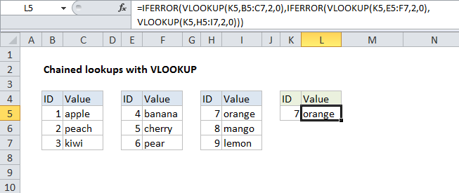
This tutorial shows how to  work  Multiple chained VLOOKUPs in Excel using the example below;

Formula

=IFERROR(VLOOKUP 1,IFERROR(VLOOKUP 2,VLOOKUP 3))
Explanation

If you need to perform multiple lookups sequentially, based on whether the earlier lookups succeed or not, you can chain one or more VLOOKUPs together with IFERROR.

Worked Example:   Create dynamic workbook reference to another workbook in Excel

In the example shown, the formula in L5 is:

=IFERROR(VLOOKUP(K5,B5:C7,2,0),IFERROR(VLOOKUP(K5,E5:F7,2,0),VLOOKUP(K5,H5:I7,2,0)))

How this formula works

The IFERROR function is designed to trap errors and perform an alternate action when an error is detected. The VLOOKUP function will throw an #N/A error when a value isn’t found.

Worked Example:   nth smallest value with criteria in Excel

By nesting multiple VLOOKUPs inside the IFERROR function, the formula allows for sequential lookups. If the first VLOOKUP fails, IFERROR catches the error and runs another VLOOKUP. If the second VLOOKUP fails, IFERROR catches the error and runs another VLOOKUP, and so on.

Worked Example:   Map inputs to arbitrary values in Excel

Post navigation

Previous Post:

Merge tables with VLOOKUP in Excel

Next Post:

Multi-criteria lookup and transpose in Excel

Leave a Reply Cancel reply

Your email address will not be published. Required fields are marked *

Learn Basic Excel

Ribbon
Workbook
Worksheets
Format Cells
Find & Select
Sort & Filter
Templates
Print
Share
Protect
Keyboard Shortcuts

Categories

  • Charts
  • Data Analysis
  • Data Validation
  • Excel Functions
    • Cube Functions
    • Database Functions
    • Date and Time Functions
    • Engineering Functions
    • Financial Functions
    • Information Functions
    • Logical Functions
    • Lookup and Reference Functions
    • Math and Trig Functions
    • Statistical Functions
    • Text Functions
    • Web Functions
  • Excel VBA
  • Excel Video Tutorials
  • Formatting
  • Grouping
  • Others
  • How to count total characters in a range in Excel
  • Extract middle name from full name — Manipulating NAMES in Excel
  • How to count specific characters in a cell in Excel
  • Convert Numbers to Text in Excel
  • How to extract word containing specific text in Excel
  • How to calculate next anniversary date or birthday in Excel
  • Get week number from date in Excel
  • Get project midpoint in Excel
  • Get days, hours, and minutes between dates in Excel
  • Sum race time splits in Excel
  • IRR function: Description, Usage, Syntax, Examples and Explanation
  • TBILLYIELD function: Description, Usage, Syntax, Examples and Explanation
  • ACCRINT function: Description, Usage, Syntax, Examples and Explanation
  • How to calculate Net Present Value (NPV) in Excel
  • RECEIVED function: Description, Usage, Syntax, Examples and Explanation
Acronyms, Abbreviations, Initialism & What They Stand For
© 2022 xlsoffice . All Right Reserved. | Teal Smiles