Lookup with variable sheet name in Excel

This tutorial shows how to Lookup with variable sheet name in Excel using the example below;

Formula

=VLOOKUP(val,INDIRECT("'"&sheet&"'!"&"range"),col,0)

Explanation

To create a lookup with a variable sheet name, you can use the VLOOKUP function together with the INDIRECT function.

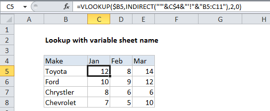
In the example shown, the formula in C5 is:

=VLOOKUP($B5,INDIRECT("'"&C$4&"'!"&"B5:C11"),2,0)

How this formula works

The “month” tabs of the worksheet contain a table that looks like this:

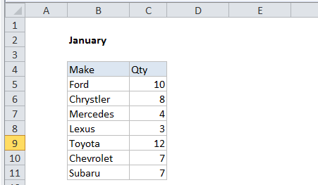
The VLOOKUP formulas on the summary tab lookup and extract data from the month tabs, by creating a dynamic reference to the sheet name for each month.

The lookup value is entered as the mixed reference $B5, with the column locked to allow copying across the table.

The table_array is created using the INDIRECT function like this:

INDIRECT("'"&C$4&"'!B5:C11")

The mixed reference C$4 refers to the column headings in row 4, which match sheet names in the workbook (i.e. “Jan”, “Feb”, “Mar”).

A single quote character is joined to either side of C$4 using the concatenation operator (&). This is not required in this particular example, but it allows the formula to handle sheet names with spaces.

Next, the exclamation point (!) is joined on the right to create a proper sheet reference, which is followed by the actual range for the table array.

Finally, inside VLOOKUP, 2 is provided for column index with 0 to force an exact match.