Lookup last file version in Excel

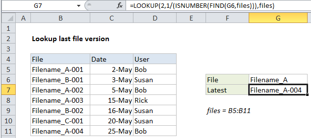
To lookup the latest file version in a list, you can use a formula based on the LOOKUP function together with the ISNUMBER and FIND functions. In the example shown, the formula in cell G7 is:

=LOOKUP(2,1/(ISNUMBER(FIND(G6,files))),files)

where “files” is the named range B5:B11.

Context

In this example, we have a number of file versions listed in a table with a date and user name. Note that file names are repeated with a counter at the end as a revision number – 001, 002, 003, etc.

Given a file name, we want to retrieve the name of the last or latest revision. There are two challenges:

1. The challenge is the version codes at the end of the file names make it harder to match the file name.
2. By default, Excel match formulas will return the first match, not the last match.

To overcome these challenges, we need to use some tricky techniques.

How this formula works

This formula uses the LOOKUP function to find and retrieve the last matching file name. The lookup value is 2, and the lookup_vector is created with this:

1/(ISNUMBER(FIND(G6,files)))

Inside this snippet, the FIND function looks for the value in G6 inside the named range “files” (B5:B11). The result is an array like this:

{1;#VALUE!;1;1;#VALUE!;#VALUE!;1}

Here, the number 1 represents a match, and the #VALUE error represents a non-matching file name. This array goes into the ISNUMBER function and comes out like this:

{TRUE;FALSE;TRUE;TRUE;FALSE;FALSE;TRUE}

Error values are now FALSE, and the number 1 is now TRUE. This overcomes challenge #1, we now have an array that shows clearly which files in the list contain the file name of interest.

Next, the array is used as the denominator with 1 as numerator. The result looks like this:

{1;#DIV/0!;1;1;#DIV/0!;#DIV/0!;1}

which goes into LOOKUP as the lookup_vector. This is a tricky solution to challenge #2. The LOOKUP function operates in approximate match mode only, and automatically ignores error values. This means with 2 as a lookup value, VLOOKUP will try to find 2, fail, and step back to the previous number (in this case matching the last 1 in position 7). Finally, LOOKUP uses 7 like an index to retrieve the 7th file in the list of files.

Handling blank lookups

Oddly, the FIND function returns 1 if the lookup value is an empty string (“”). To guard against a false match, you can wrap the formula in IF and test for an empty lookup:

=IF(G6<>"",LOOKUP(2,1/(ISNUMBER(FIND(G6,files))),files),"")