How To Insert, Edit Show or Hide Comments

You can insert a comment in Excel to give feedback about the content of a cell.

Insert Comment

To insert a comment, execute the following steps.

1. Select a cell.

2. Right click, and then click Insert Comment.

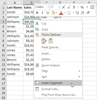
3. Type your comment.

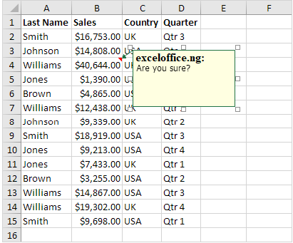
Excel displays a red triangle in the upper-right corner of the cell.

4. Click outside the comment box.

5. Hover over the cell to view the comment.

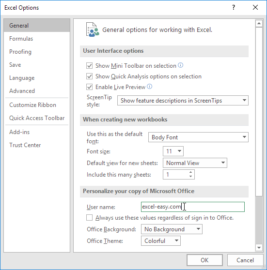
Excel automatically adds your user name. To change this name, execute the following steps.

6. On the File tab, click Options.

7. Change the User name.

Edit Comment

To edit a comment, execute the following steps.

1. Select the cell with the comment you want to edit.

2. Right click, and then click Edit Comment.

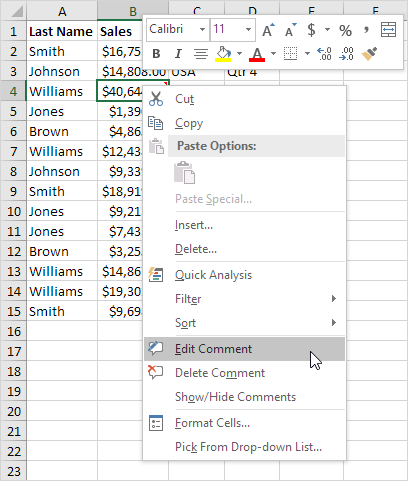
3. Edit the comment.

Note: To delete a comment, click Delete Comment.

Show/Hide Comment

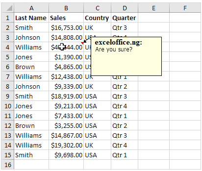
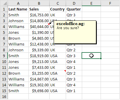
By default, a comment is only visible when you hover over the cell that contains the comment. To keep a comment visible all the time, execute the following steps.

1. For example, select cell B4 below.

2. On the Review tab, in the Comments group, click Show/Hide Comment.

3. Select another cell.

Note: to hide the comment, select cell B4 and click Show/Hide Comment again. To keep all comments visible all the time, click Show All Comments.