Count if row meets multiple internal criteria in Excel

This tutorial shows how to Count if row meets multiple internal criteria in Excel using the example below;

Formula

=SUMPRODUCT((logical1)*(logical2))

Explanation

To count rows in a table that meet multiple criteria, some of which depends on logical tests that work at the row-level, you can use the SUMPRODUCT function.

Context

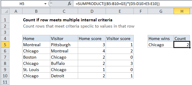
You have a table that contains the results of sports matches. You have four columns: home team, visiting team, home team score, visiting team score. For a given team, you want to count only matches (rows) where the team won at home. It’s easy to count matches (rows) where a team was the home team, but how do you count only wins?

This is a good use of the SUMPRODUCT function, which can handle array operations (think operations that deal with ranges) natively.

In the example shown, the formula in cell H5 is:

=SUMPRODUCT((B5:B10=G5)*(D5:D10>E5:E10))

How this formula works

The SUMPRODUCT function is programmed to handle arrays natively, without requiring Control Shift Enter. It’s default behavior is to multiply corresponding elements in one or more arrays together, then sum the products. When given a single array, it returns the sum of the elements in the array.

In this example, we are using two logical expressions inside a single array argument. We could place each expression into a separate argument, but then we’d need to coerce logical TRUE FALSE values to ones and zeros with another operator.

By using the multiplication operator to multiply the two arrays together, Excel will automatically coerce logical values to ones and zeros.

After the two logical expressions are evaluated, the formula looks like this:

=SUMPRODUCT(({FALSE;TRUE;FALSE;TRUE;FALSE;TRUE})*({TRUE;TRUE;TRUE;FALSE;TRUE;TRUE}))

After the two arrays are multiplied, the formula looks like this:

=SUMPRODUCT({0;1;0;0;0;1})

With only one array remaining, SUMPRODUCT simply adds up the elements in the array and returns the sum.