Circular Reference Problem Solved

You’ve entered a formula, but it’s not working. Instead, you’ve got this message about a “circular reference.”

Circular Reference occurs your formula is trying to calculate itself.

A formula in a cell that directly or indirectly refers to its own cell is called a circular reference.

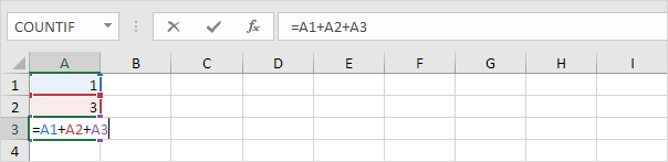
1. For example, the formula in cell A3 below directly refers to its own cell.

Remove or allow a circular reference

Trying to calculate itself. To fix the problem, you can move the formula to another cell (in the formula bar, press Ctrl+X to cut the formula, select another cell, and press Ctrl+V).

Note: Excel returns a 0 if you accept this circular reference.

 

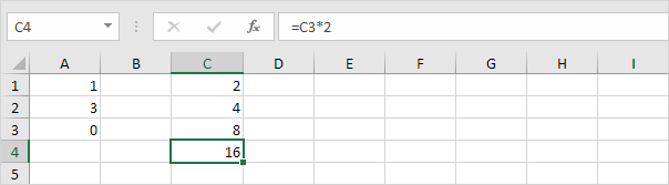
2a. For example, the formula in cell C2 below refers to cell C1.

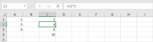
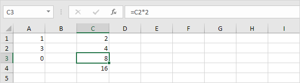
2b. The formula in cell C3 refers to cell C2.

2c. The formula in cell C4 refers to cell C3.

2d. So far, everything’s OK. Now change the value in cell C1 to the formula =C4. Cell C1 refers to cell C4, cell C4 refers to cell C3, cell C3 refers to cell C2, and cell C2 refers to cell C1. In other words, the formula in cell C1 indirectly refers to its own cell. This is not possible.

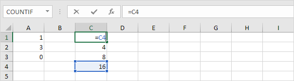
Note: Excel returns a 0 if you accept this circular reference.

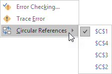
3. To find your circular references, on the Formulas tab, in the Formula Auditing group, click the down arrow next to Error Checking.

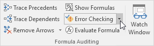
4. Click Circular References.