Average and ignore errors in Excel

This tutorial shows how to work Average and ignore errors in Excel using the example below;

Formula

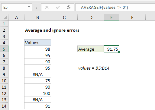
=AVERAGEIF(values,">=0")

Explanation

To average a list of values, ignoring any errors that might exist in the range, you can use the AVERAGEIF or AGGREGATE function, as described below. In the example shown, the formula in E5 is:

=AVERAGEIF(values,">=0")

where “values” is the named range B5:B14.

How this formula works

The AVERAGEIF function can calculate an average of numeric data with one or more criteria. In this case, the criteria is the expression “>=0”. This filters out error values, and AVERAGEIF returns the average of the remaining eight values, 91.75.

Alternative with AGGREGATE

The AGGREGATE function can also ignore errors when calculating an average. To calculate an average with the AGGREGATE function, you can use a formula like this:

=AGGREGATE(1,6,values)

Here, the number 1 specifies average, and the number 6 is an option to ignore errors. Like AVERAGEIF above, AGGREGATE returns the average of the remaining eight values, 91.75.