Add Leading Zeros, Text And Colours Custom Number Format

Excel Custom Number Format with Leading Zeros, Add Text, Colours Example

How to add a leading zero in excel

Beyond the built-in options: The Format Cells dialog offers so many options available “out-of-the-box.” The available format category and type options go far beyond the basics.

But, if what is available still doesn’t meet your requirements, you can always create a custom format.

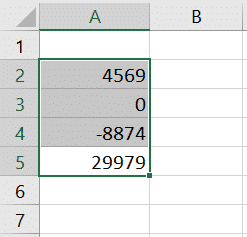
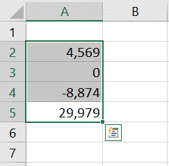
Let’s consider a set of numbers.

We start by opening the Format Cells dialog box as we did before. This time we will select Custom from the Category list.

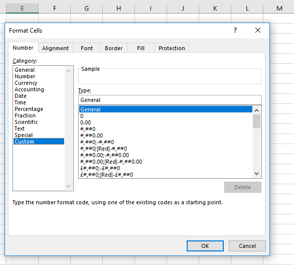
Then we select from the Type list.

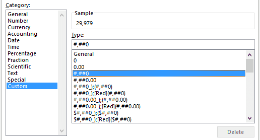
We will start with “#,##0” and then build our own custom format from there.

If we want to build our own custom currency format, one of the first things we can do is add a dollar sign.

We can type that into the Type text box.

One of the things you can customize is the colour of your type font.

You do this by preceding your number format with the colour name enclosed in square brackets.

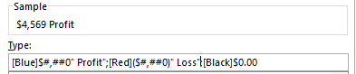
We add blue type font formatting to our current format.

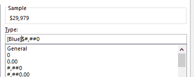
The preview in the Sample box does not show colour changes.

We must click OK to see the change.

So far, we have only worked with number formats that consist of one section of code.

Using semicolons to separate, we can have up to four of these code sections.

This means that we can do something like format both positive and negative numbers.

For instance, we may want our negative numbers to show up red font. This will be a good contrast to the blue we have set for positive numbers.

We could also have negative numbers shown in parentheses.

We can even go a step further and set a third code section for zero values.

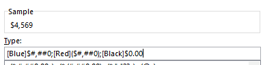
This will now change our list of numeric values to something more meaningful.

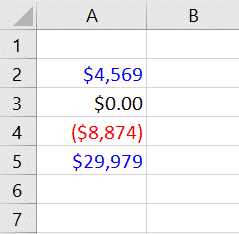
This is a great demonstration of the flexibility custom number formatting offers. But let’s go even a step further.

Custom formatting even allows you to add text to your formats.

You could be even more descriptive based on whether your values are positive or negative.

You can do this by adding text by enclosing the custom string in double quotes.

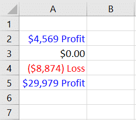
We have added the text “ Profit” to the end of our positive values. We have also added the text “ Loss” to the end of our negative values.

Pay attention to the spaces after the opening double quote and the first letter of each string.

Without these leading spaces, there would be no space between the numeric value and the text.

Now our updated custom format codes yield the following results.

Example: Decimal Places Custom Format in Excel

You can control the number of decimal places. Use 0 to display the nearest integer value. Use 0.0 for one decimal place. Use 0.00 for two decimal places, etc.

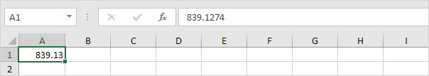
1. Enter the value 839.1274 into cell A1.

2. Use the following number format code: 0.00

Example: Add Leading Zeros in Excel

For example, you might have codes that consist of 5 numbers. Instead of typing 00041, simply type 41 and let Excel add the leading zeros.

1. Enter the value 41 into cell A1.

2. Select cell A1, right click, and then click Format Cells.

3. Select Custom.

4. Type the following number format code: 00000

5. Click OK.

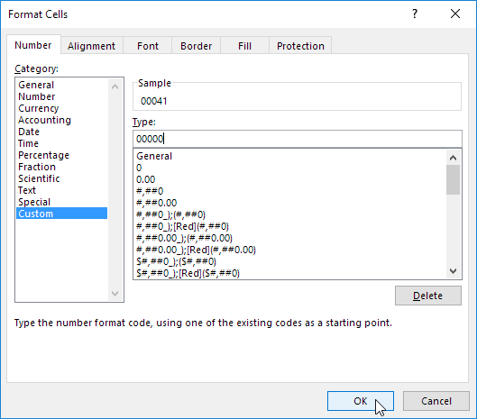
Note: Excel gives you a life preview of how the number will be formatted (under Sample).

Result:

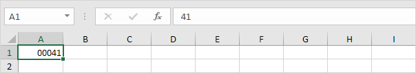
Note: cell A1 still contains the number 41. We only changed the appearance of this number, not the number itself.

Example: Add Text Custom Format in Excel

You can also add text to your numbers. For example, add “ft”.

1. Enter the value 839.1274 into cell A1.

2. Use the following number format code: 0.0 “ft”

Note: remember, we only changed the appearance of this number, not the number itself. You can still use this number in your calculations.

Example: Large Numbers Custom Format in Excel

You can also control large numbers. Use one comma (,) to display thousands and use two commas (,,) to display millions.

1. Enter the following values in cells A1, B1, C1 and D1: 1000000, 2500000, 81000000 and 700000.

2. Use the following number format code: 0.0,, “M”

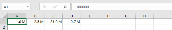
Note: we used 0.0 for one decimal place and “M” to add the letter M.

Example: Add Colour Custom Number Format in Excel

You can control positive numbers, negative numbers, zero values and text all at the same time! Each part is separated with a semicolon (;) in your number format code.

1. Enter the following values in cells A1, B1, C1 and A2: 5000000, 0, Hi and -5.89.

2. Use the following number format code: [Green]$#,##0_);[Red]$(#,##0);”zero”;[Blue]”Text:” @

Note: #,## is used to add comma’s to large numbers. To add a space, use the underscore “_” followed by a character. The length of the space will be the length of this character. In our example, we added a parentheses “)”. As a result, the positive number lines up correctly with the negative number enclosed in parentheses. Use two parts separated with a semicolon (;) to control positive and negative numbers only. Use three parts separated with a semicolon (;) to control positive numbers, negative numbers and zero values only.

Example: Custom Dates and Times Format in Excel

You can also control dates and times. Use one of the existing Date or Time formats as a starting point.

1. Enter the value 42855 into cell A1.

2. Select cell A1, right click, and then click Format Cells.

3. Select Date and select the Long Date.

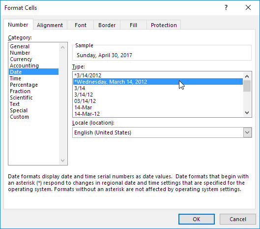
Note: Excel gives you a life preview of how the number will be formatted (under Sample).

4. Select Custom.

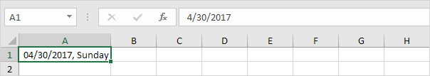
5. Slightly change the number format code to: mm/dd/yyyy, dddd

6. Click OK.

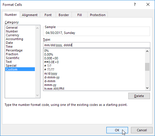
Result:

Example: Repeat Characters Custom Format in Excel

Use the asterisk (*) followed with a character to fill a cell with that character.

1. Type Hi into cell A1.

2. Use the following number format code: @ *-

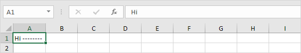
Note: the @ symbol is used to get the text input.