Conditional formatting column is blank in Excel

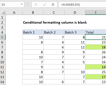
This tutorial shows how to Conditionally format column is blank in Excel using the example below;

Formula

=OR(A1="",B1="", C1="")

Explanation

To highlight values in one column when values in one or more other columns are blank, you can use the OR function and a basic logical expression to test for blank or empty values. In the example shown, conditional formatting has been applied to the range E5:E14 with this formula:

=OR(B5="",C5="", D5="")

If B5 or C5 or D5 is blank, the formula returns TRUE and triggers the rule.

Note: conditional formatting formulas should be entered relative to the “active cell” in the selection, which is assumed to be E5 in this case.

How this formula works

When conditional formatting is applied with a formula, the formula is evaluated relative to the active cell in the selection at the time the rule is created. In this case, the active cell when the rule is created is assumed to be cell E5, with the range E5:E14 selected.

As the formula is evaluated, formula references change so that the rule is testing for blank values in the correct row for each of the 10 cells in the range:

=OR(B5="",C5="", D5="") // E5
=OR(B6="",C6="", D6="") // E6
=OR(B7="",C7="", D7="") // E7
etc.

If any cell in a corresponding row in column B, C, or D is blank, OR function returns TRUE and the rule is triggered and the green fill is applied. When all tests return FALSE, the OR function returns FALSE and no conditional formatting is applied.

With ISBLANK

of testing for an empty string (=””) directly you can use the ISBLANK function in an equivalent formula like this:

=OR(ISBLANK(B5),ISBLANK(C5),ISBLANK(D5))

AND, OR, NOT

Other logical tests can be constructed using combinations of AND, OR, and NOT. For example, to test for a blank cell in column B and column D, you could use a formula like this:

=AND(B5="",D5="")

This will trigger conditional formatting only when the column B and D are blank.