Skip to content
xlsoffice. All Rights Reserved
  • Home
  • Excel For Beginners
  • Excel Intermediate
  • Advanced Excel For Experts

Lookup and Reference Examples

  • Merge tables with VLOOKUP in Excel
  • How to get relative column numbers in a range in Excel
  • Two-column Lookup in Excel
  • Basic INDEX MATCH approximate in Excel
  • Create hyperlink with VLOOKUP in Excel

Data Analysis Examples

  • How to count table columns in Excel
  • Chart Axes in Excel
  • Managing Conditional Formatting Rules in Excel
  • How to create running total in an Excel Table
  • How To Remove Duplicates In Excel Column Or Row?

Data Validation Examples

  • Excel Data validation date in next 30 days
  • Excel Data validation must begin with
  • Excel Data validation allow uppercase only
  • How To Create Drop-down List in Excel
  • Data validation must not exist in list

How to Separate Text Strings in Excel

by

This example teaches you how to separate strings in Excel. Asides from using ‘Convert Text to Columns Wizard’ in data tab, you can as well follow the steps below to Separate Text Strings in Excel .

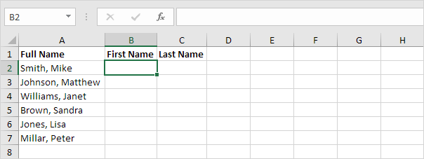
The problem we are dealing with is that we need to tell Excel where we want to separate the string. In case of Smith, Mike the comma is at position 6 while in case of Williams, Janet the comma is at position 9.

Worked Example:   Floating Point Errors in Excel

1. To get the first name, use the formula below.

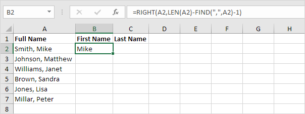
Explanation: to find the position of the comma, use the FIND function (position 6). To get the length of a string, use the LEN function (11 characters). =RIGHT(A2,LEN(A2)-FIND(“,”,A2)-1) reduces to =RIGHT(A2,11-6-1). =RIGHT(A2,4) extracts the 4 rightmost characters and gives the desired result (Mike).

Worked Example:   Excel Functions by Categories

2. To get the last name, use the following formula.

Worked Example:   How to strip non-numeric characters in Excel

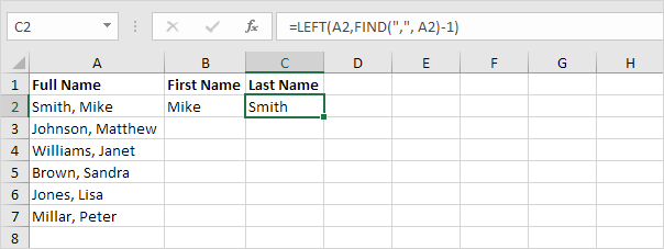
Explanation: to find the position of the comma, use the FIND function (position 6). =LEFT(A2,FIND(“,”, A2)-1) reduces to =LEFT(A2,6-1). =LEFT(A2,5) extracts the 5 leftmost characters and gives the desired result (Smith).

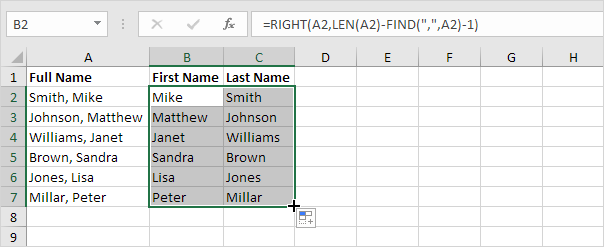
3. Select the range B2:C2 and drag it down.

Post navigation

Previous Post:

How to calculate Number of Instances in Excel

Next Post:

How to calculate Quarter of Date in Excel

Leave a Reply Cancel reply

Your email address will not be published. Required fields are marked *

Learn Basic Excel

Ribbon
Workbook
Worksheets
Format Cells
Find & Select
Sort & Filter
Templates
Print
Share
Protect
Keyboard Shortcuts

Categories

  • Charts
  • Data Analysis
  • Data Validation
  • Excel Functions
    • Cube Functions
    • Database Functions
    • Date and Time Functions
    • Engineering Functions
    • Financial Functions
    • Information Functions
    • Logical Functions
    • Lookup and Reference Functions
    • Math and Trig Functions
    • Statistical Functions
    • Text Functions
    • Web Functions
  • Excel VBA
  • Excel Video Tutorials
  • Formatting
  • Grouping
  • Others
  • REPT function: Description, Usage, Syntax, Examples and Explanation
  • Convert text to numbers using VALUE function in Excel
  • EXACT function: Description, Usage, Syntax, Examples and Explanation
  • DBCS function: Description, Usage, Syntax, Examples and Explanation
  • Find most frequent text within a range with criteria in Excel
  • Get day from date in Excel
  • Add days exclude certain days of week in Excel
  • Pad week numbers with zeros in Excel
  • YEARFRAC function: Description, Usage, Syntax, Examples and Explanation
  • Basic timesheet formula with breaks in Excel
  • XIRR function: Description, Usage, Syntax, Examples and Explanation
  • Calculate original loan amount in Excel
  • PRICEMAT function: Description, Usage, Syntax, Examples and Explanation
  • Calculate payment for a loan in Excel
  • ODDLYIELD function: Description, Usage, Syntax, Examples and Explanation
Acronyms, Abbreviations, Initialism & What They Stand For
© 2021 xlsoffice. All Rights Reserved | Teal Smiles