Skip to content
Free Excel Tutorials
  • Home
  • Excel For Beginners
  • Excel Intermediate
  • Advanced Excel For Experts

Data Analysis

  • Reverse List in Excel
  • How to calculate correlation coefficient Correlation in Excel
  • Conflicting Multiple Conditional Formatting Rules in Excel
  • How to add Trendline to a chart in Excel
  • Everything about Charts in Excel

References

  • How to use Excel FORMULATEXT function
  • Find closest match in Excel
  • How to use Excel INDIRECT Function
  • How to get address of named range in Excel
  • To count total rows in a range in Excel

Data Validations

  • Excel Data validation whole percentage only
  • How To Create Drop-down List in Excel
  • Excel Data validation must contain specific text
  • Excel Data validation date in specific year
  • Excel Data validation must begin with

Extract last name from full name — Manipulating NAMES in Excel

by

If you need extract the last name from a full name, you can do so with this rather complex formula that uses several functions.

Note: In the  formula below, name is a full name, with a space separating the first name from other parts of the name.

Formula

=RIGHT(name,LEN(name)-FIND("*",SUBSTITUTE(name," ","*",
LEN(name)-LEN(SUBSTITUTE(name," ","")))))
Extract last name from full name -- Manipulating NAMES in Excel

Important!

Handling inconsistent spaces

Extra spaces will cause problems with this formula. One solution is to use the TRIM function first to clean things up, then use the parsing formula.

Explanation

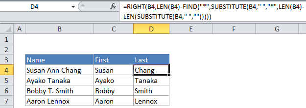
In the example, the active cell contains this formula:

=RIGHT(B4,LEN(B4)-FIND("*",SUBSTITUTE(B4," ","*",LEN(B4)-LEN(SUBSTITUTE(B4," ","")))))

How this formula works

At the core, this formula uses the RIGHT function to extract characters starting from the right. The other functions which make up the complex part of this formula just do one thing: they calculate how many characters need to be extracted.

At a high level, the formula replaces the last space in the name with an asterisk “*” and then uses FIND to determine the position of the asterisk in the name. The position is used to work out how many characters to extract with RIGHT.

How does the function replace only the last space? This is the clever part.

Buckle up, the explanation gets a bit technical.

They key to this formula is this bit:

SUBSTITUTE(B4," ","*",LEN(B4)-LEN(SUBSTITUTE(B4," ","")))

Which does the actual replacement of the last space with “*”.

SUBSTITUTE has a forth (optional) argument that specifies which “instance” of the find text should be replaced. If nothing is supplied for this argument, all instances are replaced. However, if, say the number 2 is supplied, only the second instance is replaced. In the snippet above, instance is calculated using the second SUBSTITUTE:

LEN(B4)-LEN(SUBSTITUTE(B4," ",""))

Here, the length of the name without any spaces is subtracted from the actual length of the name. If there’s only one space in the name, it produces 1. If there are two spaces, it the result is 2, and so on.

In the example name in B4, there are two spaces in the name, so we get:

15 – 13 = 2

And two is used as in the instance number:

SUBSTITUTE(B4," ","*",2)

which replaces the second space with “*”. The name then looks like this:

“Susan Ann*Chang”

The FIND function then takes over to figure out where the “*” is in the name:

FIND("*", "Susan Ann*Chang")

The result is 10 (the * is in the 10th position) which is subtracted from the total length of the name:

LEN(B4)-10

Since the name is 15 characters, we have:

15-10 = 5

The number 5 is used by RIGHT like so:

=RIGHT(B4,5)

Which results in “Chang”

As, you can see, it’s a lot of work above to calculate that simple 5!

Post navigation

Next Post:

Create One-dimensional and Two-dimensional Array

Leave a Reply Cancel reply

Your email address will not be published. Required fields are marked *

Learn Basic Excel

Ribbon
Workbook
Worksheets
Format Cells
Find & Select
Sort & Filter
Templates
Print
Share
Protect
Keyboard Shortcuts

Categories

  • Charts
  • Data Analysis
  • Data Validation
  • Excel Functions
    • Cube Functions
    • Database Functions
    • Date and Time Functions
    • Engineering Functions
    • Financial Functions
    • Information Functions
    • Logical Functions
    • Lookup and Reference Functions
    • Math and Trig Functions
    • Statistical Functions
    • Text Functions
    • Web Functions
  • Excel VBA
  • Excel Video Tutorials
  • Formatting
  • Grouping
  • Others

Logical Functions

  • IFERROR function: Description, Usage, Syntax, Examples and Explanation
  • Nested IF function example in Excel
  • SWITCH function example in Excel
  • How to return blank in place of #DIV/0! error in Excel
  • IFNA function: Description, Usage, Syntax, Examples and Explanation

Date Time

  • Display Days until expiration date in Excel
  • Calculate date overlap in days in Excel
  • Calculate years between dates in Excel
  • Basic Overtime Calculation Formula in Excel
  • How to get same date next year or previous year in Excel

Grouping

  • Calculate conditional mode with criteria in Excel
  • Categorize text with keywords in Excel
  • Group numbers with VLOOKUP in Excel
  • How to randomly assign data to groups in Excel
  • If cell contains one of many things in Excel

General

  • How to password protect excel sheet?
  • Split Cell Content Using Text to Columns in Excel
  • Share Excel data with Word documents
  • Find Most Frequently Occurring Word in Excel Worksheet
  • List worksheet index numbers in Excel
© 2025 xlsoffice . All Right Reserved. | Teal Smiles | Abbreviations And Their Meaning