
Skip to content
Free Excel Tutorials
  • Home
  • Excel For Beginners
  • Excel Intermediate
  • Advanced Excel For Experts

Data Analysis

  • Working With Tables in Excel
  • Use Data Form to input, edit and delete records in Excel
  • Understanding Pivot Tables in Excel
  • Excel Pie Chart
  • How to add Trendline to a chart in Excel

References

  • How to get last row in text data in Excel
  • Lookup entire row in Excel
  • Find closest match in Excel
  • Two-way lookup with VLOOKUP in Excel
  • How to get address of last cell in range in Excel

Data Validations

  • Excel Data validation exists in list
  • Excel Data validation don’t exceed total
  • Excel Data validation must begin with
  • Excel Data validation must contain specific text
  • Excel Data validation no punctuation

Add line break based on OS in Excel

by

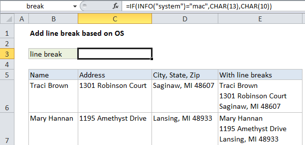
To add a line break taking into account the current OS (Mac or Windows), you can use the INFO function to test the system and then return the correct break character — CHAR(10) for Windows, CHAR(13) for Mac.

Note: make sure you have text wrap enabled on cells that contain line breaks.

Formula

=IF(INFO("system")="mac",CHAR(13),CHAR(10))
Explanation

The character used for line breaks is different depending on whether Excel is running on Mac or Windows: CHAR(10) for Windows, CHAR(13) for Mac. This makes it tricky to write a single formula that will work as expected on both platforms.

The solution is to use the INFO function to test the current environment, then adjust the line break character accordingly. We do this by adding this formula to C3:

=IF(INFO("system")="mac",CHAR(13),CHAR(10))

Then we we name C3 “break” so we can use the word break like a variable later. If Excel is running on a Mac, break will equal CHAR(13), if not, break will equal CHAR(10).

In column E, we concatenate the address information that appears in B, C, and D with a formula like this:

=B6&break&C6&break&D6

The result of the concatenation is text with line breaks:

Traci Brown¬
1301 Robinson Court¬
Saginaw, MI 48607


Post navigation

Previous Post:

DECIMAL function: Description, Usage, Syntax, Examples and Explanation

Next Post:

AVERAGE function: Description, Usage, Syntax, Examples and Explanation

Leave a Reply Cancel reply

Your email address will not be published. Required fields are marked *

Learn Basic Excel

Ribbon
Workbook
Worksheets
Format Cells
Find & Select
Sort & Filter
Templates
Print
Share
Protect
Keyboard Shortcuts

Categories

  • Charts
  • Data Analysis
  • Data Validation
  • Excel Functions
    • Cube Functions
    • Database Functions
    • Date and Time Functions
    • Engineering Functions
    • Financial Functions
    • Information Functions
    • Logical Functions
    • Lookup and Reference Functions
    • Math and Trig Functions
    • Statistical Functions
    • Text Functions
    • Web Functions
  • Excel VBA
  • Excel Video Tutorials
  • Formatting
  • Grouping
  • Others

Logical Functions

  • IF with boolean logic in Excel
  • How to use IFS function in Excel
  • How to return blank in place of #DIV/0! error in Excel
  • IF, AND, OR and NOT Functions Examples in Excel
  • How to use Excel XOR Function

Date Time

  • Count times in a specific range in Excel
  • DATEVALUE function: Description, Usage, Syntax, Examples and Explanation
  • Get days, hours, and minutes between dates in Excel
  • DATE function: Description, Usage, Syntax, Examples and Explanation
  • Count holidays between two dates in Excel

Grouping

  • Group numbers with VLOOKUP in Excel
  • Calculate conditional mode with criteria in Excel
  • How to randomly assign people to groups in Excel
  • How to randomly assign data to groups in Excel
  • If cell contains one of many things in Excel

General

  • AutoFit Column Width, AutoFit Row Height in Excel
  • List worksheet index numbers in Excel
  • Sum by group in Excel
  • How to calculate percentage of total in Excel
  • Find, Select, Replace and Go To Special in Excel
© 2026 xlsoffice . All Right Reserved. | Teal Smiles | Abbreviations And Their Meaning