
Conditional Formatting Rules in Excel
Quickly identify variances in record using Conditional formatting.
Conditional formatting in Excel enables you to highlight cells with a certain color, depending on the cell’s value. By conditional formatting to your data, you can quickly identify variances in a range of values with a quick glance.
Navigation: Home Tab → Styles Group → Conditional Formating
Highlight Cells Rules
To highlight cells that are greater than a value, execute the following steps.
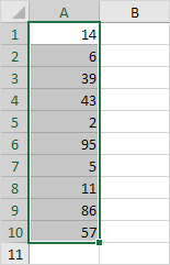
1. Select the range A1:A10.
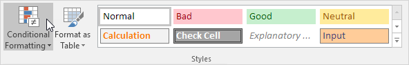
2. On the Home tab, in the Styles group, click Conditional Formatting.
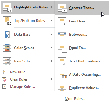
3. Click Highlight Cells Rules, Greater Than.
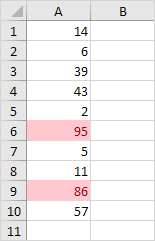
4. Enter the value 80 and select a formatting style.
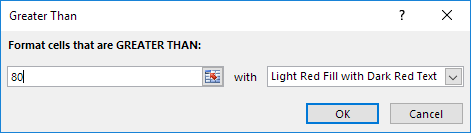
5. Click OK.
Result. Excel highlights the cells that are greater than 80.
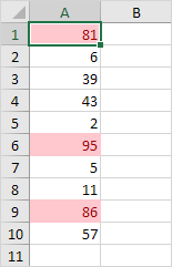
6. Change the value of cell A1 to 81.
Result. Excel changes the format of cell A1 automatically.
Note: you can also highlight cells that are less than a value, between a low and high value, etc.
Clear Rules
To clear a conditional formatting rule, execute the following steps.
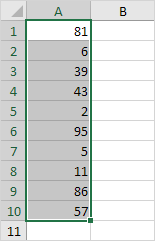
1. Select the range A1:A10.
2. On the Home tab, in the Styles group, click Conditional Formatting.
3. Click Clear Rules, Clear Rules from Selected Cells.
![]()
Top/Bottom Rules
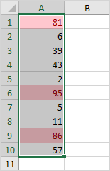
To highlight cells that are above the average of the cells, execute the following steps.
1. Select the range A1:A10.
2. On the Home tab, in the Styles group, click Conditional Formatting.
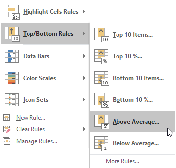
3. Click Top/Bottom Rules, Above Average.
4. Select a formatting style.
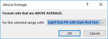
5. Click OK.
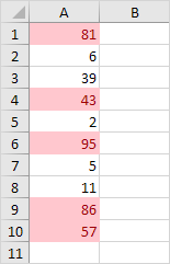
Result. Excel calculates the average (42.5) and formats the cells that are above this average.
Note: you can also highlight the top 10 items, the top 10 %, etc. The sky is the limit!