How To Filter Data in Excel

Filter your Excel data if you only want to display records that meet certain criteria.

By filtering data in a worksheet, you can find values quickly. You can filter on one or more columns of data. With filtering, you can control not only what you want to see, but what you want to exclude. You can filter based on choices you make from a list, or you can create specific filters to focus on exactly the data that you want to see.

Navigation: Data Tab → Sort & Filter Group → Filter

1. Click any single cell inside a data set.

2. On the Data tab, in the Sort & Filter group, click Filter.

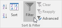
Arrows in the column headers appear.

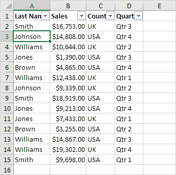
3. Click the arrow next to Country.

4. Click on Select All to clear all the check boxes, and click the check box next to USA.

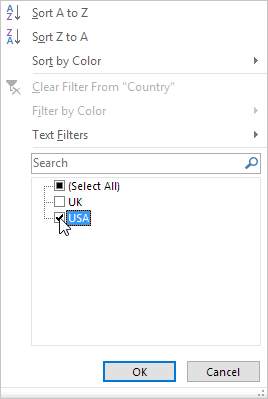
5. Click OK.

Result. Excel only displays the sales in the USA.

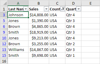
6. Click the arrow next to Quarter.

7. Click on Select All to clear all the check boxes, and click the check box next to Qtr 4.

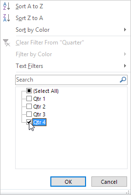
8. Click OK.

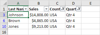
Result. Excel only displays the sales in the USA in Qtr 4.

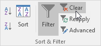
9. To remove the filter, on the Data tab, in the Sort & Filter group, click Clear. To remove the filter and the arrows, click Filter.