
Skip to content
Free Excel Tutorials
  • Home
  • Excel For Beginners
  • Excel Intermediate
  • Advanced Excel For Experts

Data Analysis

  • Calculate Conditional Percentile ‘IF’ in table in Excel
  • What-If Analysis: Scenarios and Goal Seek in Excel
  • Excel Line Chart
  • Excel Frequency Function Example
  • How To Insert and Customize Sparklines in Excel

References

  • Two-way lookup with VLOOKUP in Excel
  • Complete List of Excel Lookup and Reference Functions, References and Examples
  • How to get relative column numbers in a range in Excel
  • CHOOSE function: Description, Usage, Syntax, Examples and Explanation
  • How to get first column number in range in Excel

Data Validations

  • Excel Data validation date in next 30 days
  • Excel Data validation whole percentage only
  • Excel Data validation unique values only
  • Excel Data validation must begin with
  • Excel Data validation specific characters only

Get location of value in 2D array in Excel

by

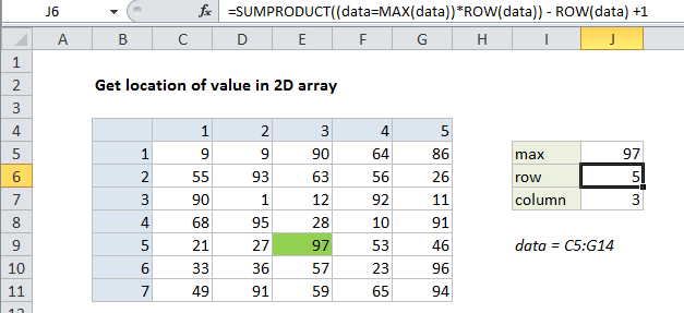
This tutorial shows how to Get location of value in 2D array in Excel using the example below;

Formula

=SUMPRODUCT((data=MAX(data))*ROW(data))-ROW(data)+1
Explanation

To locate the position of a value in a 2D array, you can use the SUMPRODUCT function. In the example shown, the formulas used to locate the row and column numbers of the max value in the array are:

=SUMPRODUCT((data=MAX(data))*ROW(data))-ROW(data)+1
=SUMPRODUCT((data=MAX(data))*COLUMN(data))-COLUMN(data)+1

where “data” is the named range C5:G14.

Note: for this example, we are arbitrarily find the location of the maximum value in the data, but you can replace data=MAX(data) with any other logical test that will isolate a given value.  Also note these formulas will fail if there are duplicate values in the array.

How these formula work

To get the row number, the data is compared to the max value, which generates an array of TRUE FALSE results. These are multiplied by the result of ROW (data) which generates and array of row numbers associated with the named range “data”:

=SUMPRODUCT({FALSE,FALSE,FALSE,FALSE,FALSE;FALSE,FALSE,FALSE,FALSE,FALSE;FALSE,FALSE,FALSE,FALSE,FALSE;FALSE,FALSE,FALSE,FALSE,FALSE;FALSE,FALSE,TRUE,FALSE,FALSE;FALSE,FALSE,FALSE,FALSE,FALSE;FALSE,FALSE,FALSE,FALSE,FALSE}*{5;6;7;8;9;10;11})

The multiplication operation causes Excel to coerce the TRUE FALSE values in the first array to 1s and 0s, so we can visualize an intermediate step like this:

=SUMPRODUCT({0,0,0,0,0;0,0,0,0,0;0,0,0,0,0;0,0,0,0,0;0,0,1,0,0;0,0,0,0,0;0,0,0,0,0}*{5;6;7;8;9;10;11})

SUMPRODUCT then returns a result of 9, which corresponds to the 9th row on the worksheet. To get an index relative to the named range “data”, we use:

-ROW(data)+1

The final result is the array {5;4;3;2;1;0;-1}, from which only the first value (5) is displayed.

The formula to determine the column position works in the same way.

Post navigation

Previous Post:

COSH function: Description, Usage, Syntax, Examples and Explanation

Next Post:

Excel Data validation require unique number

Leave a Reply Cancel reply

Your email address will not be published. Required fields are marked *

Learn Basic Excel

Ribbon
Workbook
Worksheets
Format Cells
Find & Select
Sort & Filter
Templates
Print
Share
Protect
Keyboard Shortcuts

Categories

  • Charts
  • Data Analysis
  • Data Validation
  • Excel Functions
    • Cube Functions
    • Database Functions
    • Date and Time Functions
    • Engineering Functions
    • Financial Functions
    • Information Functions
    • Logical Functions
    • Lookup and Reference Functions
    • Math and Trig Functions
    • Statistical Functions
    • Text Functions
    • Web Functions
  • Excel VBA
  • Excel Video Tutorials
  • Formatting
  • Grouping
  • Others

Logical Functions

  • IFS function: Description, Usage, Syntax, Examples and Explanation
  • Check multiple cells are equal in Excel
  • How to use Excel AND Function
  • Invoice status with nested if in Excel
  • NOT function: Description, Usage, Syntax, Examples and Explanation

Date Time

  • Get first day of previous month in Excel
  • EOMONTH function: Description, Usage, Syntax, Examples and Explanation
  • WORKDAY.INTL function: Description, Usage, Syntax, Examples and Explanation
  • Calculate retirement date in Excel
  • Create date range from two dates in Excel

Grouping

  • How to randomly assign people to groups in Excel
  • Running count group by n size in Excel
  • Group arbitrary text values in Excel
  • Map text to numbers in Excel
  • Group numbers at uneven intervals in Excel

General

  • How to calculate percent change in Excel
  • Creating and Opening an existing file in Excel
  • How to choose page/paper size in Excel before Printing
  • How to fill cell ranges with random number from fixed set of options in Excel
  • How to calculate project complete percentage in Excel
© 2026 xlsoffice . All Right Reserved. | Teal Smiles | Abbreviations And Their Meaning