Sum by month ignore year in Excel
This tutorial shows how to Sum by month ignore year in Excel using the example below;
Formula
=SUMPRODUCT((MONTH(dates)=month)*amounts)
Explanation
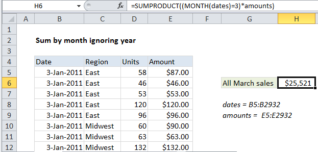
To sum data by month, ignoring year, you can use a formula based on the SUMPRODUCT and MONTH functions. In the example shown, the formula in H6 is:
=SUMPRODUCT((MONTH(dates)=3)*amounts)
The result is a total of all sales in March, ignoring year.
How this formula works
This data set contains over 2900 records, and the formula above uses two named ranges:
dates = B5:B2932
amounts =  E5:E2932
Inside the SUMPRODUCT function, the MONTH function is used to extract the month number for every date in the data set, and compare it with the number 3:
(MONTH(dates)=3)
If we assume a small data set listing 3 dates each in January, February, and March (in that order), the result would be an array containing nine numbers like this:
{1;1;1;2;2;2;3;3;3}
where each number is the “month number” for a date. When the values are compared to 3, the result is an array like this:
{FALSE;FALSE;FALSE;FALSE;FALSE;FALSE;TRUE;TRUE;TRUE}
This array is then multiplied by the amount values associated with each March date. If we assume all nine amounts are equal to 100, the operation looks like this:
{0;0;0;0;0;0;1;1;1} * {100;100;100;100;100;100;100;100;100}
Notice the math operation changes the TRUE FALSE values into ones and zeros. After multiplication, we have a single array in SUMPRODUCT:
=SUMPRODUCT({0;0;0;0;0;0;100;100;100})
Note the only surviving amounts are associated with March, the rest are zero.
Finally, SUMPRODUCT returns the sum of all items – 300 in the abbreviated example above, and 25,521 in the screenshot with actual data.
2. Count by month ignoring year
To get a count by month ignoring year, you can use SUMPRODUCT like this:
=SUMPRODUCT(--(MONTH(dates)=3))
Average by month ignoring year
To calculate and average by month ignoring year, you combine the two SUMPRODUCT formulas above like this:
=SUMPRODUCT((MONTH(dates)=3)*amounts)/SUMPRODUCT(--(MONTH(dates)=3))
formula
=SUMPRODUCT((MONTH(dates)=month)*amounts)
Explanation
To sum data by month, ignoring year, you can use a formula based on the SUMPRODUCT and MONTH functions. In the example shown, the formula in H6 is:
=SUMPRODUCT((MONTH(dates)=3)*amounts)
The result is a total of all sales in March, ignoring year.
How this formula works
This data set contains over 2900 records, and the formula above uses two named ranges:
dates = B5:B2932
amounts =  E5:E2932
Inside the SUMPRODUCT function, the MONTH function is used to extract the month number for every date in the data set, and compare it with the number 3:
(MONTH(dates)=3)
If we assume a small data set listing 3 dates each in January, February, and March (in that order), the result would be an array containing nine numbers like this:
{1;1;1;2;2;2;3;3;3}
where each number is the “month number” for a date. When the values are compared to 3, the result is an array like this:
{FALSE;FALSE;FALSE;FALSE;FALSE;FALSE;TRUE;TRUE;TRUE}
This array is then multiplied by the amount values associated with each March date. If we assume all nine amounts are equal to 100, the operation looks like this:
{0;0;0;0;0;0;1;1;1} * {100;100;100;100;100;100;100;100;100}
Notice the math operation changes the TRUE FALSE values into ones and zeros. After multiplication, we have a single array in SUMPRODUCT:
=SUMPRODUCT({0;0;0;0;0;0;100;100;100})
Note the only surviving amounts are associated with March, the rest are zero.
Finally, SUMPRODUCT returns the sum of all items – 300 in the abbreviated example above, and 25,521 in the screenshot with actual data.
3. Count by month ignoring year
To get a count by month ignoring year, you can use SUMPRODUCT like this:
=SUMPRODUCT(--(MONTH(dates)=3))
Average by month ignoring year
To calculate and average by month ignoring year, you combine the two SUMPRODUCT formulas above like this:
=SUMPRODUCT((MONTH(dates)=3)*amounts)/SUMPRODUCT(--(MONTH(dates)=3))
formula
=SUMPRODUCT((MONTH(dates)=month)*amounts)
Explanation
To sum data by month, ignoring year, you can use a formula based on the SUMPRODUCT and MONTH functions. In the example shown, the formula in H6 is:
=SUMPRODUCT((MONTH(dates)=3)*amounts)
The result is a total of all sales in March, ignoring year.
How this formula works
This data set contains over 2900 records, and the formula above uses two named ranges:
dates = B5:B2932
amounts =  E5:E2932
Inside the SUMPRODUCT function, the MONTH function is used to extract the month number for every date in the data set, and compare it with the number 3:
(MONTH(dates)=3)
If we assume a small data set listing 3 dates each in January, February, and March (in that order), the result would be an array containing nine numbers like this:
{1;1;1;2;2;2;3;3;3}
where each number is the “month number” for a date. When the values are compared to 3, the result is an array like this:
{FALSE;FALSE;FALSE;FALSE;FALSE;FALSE;TRUE;TRUE;TRUE}
This array is then multiplied by the amount values associated with each March date. If we assume all nine amounts are equal to 100, the operation looks like this:
{0;0;0;0;0;0;1;1;1} * {100;100;100;100;100;100;100;100;100}
Notice the math operation changes the TRUE FALSE values into ones and zeros. After multiplication, we have a single array in SUMPRODUCT:
=SUMPRODUCT({0;0;0;0;0;0;100;100;100})
Note the only surviving amounts are associated with March, the rest are zero.
Finally, SUMPRODUCT returns the sum of all items – 300 in the abbreviated example above, and 25,521 in the screenshot with actual data.
4. Count by month ignoring year
To get a count by month ignoring year, you can use SUMPRODUCT like this:
=SUMPRODUCT(--(MONTH(dates)=3))
5. Average by month ignoring year
To calculate and average by month ignoring year, you combine the two SUMPRODUCT formulas above like this:
=SUMPRODUCT((MONTH(dates)=3)*amounts)/SUMPRODUCT(--(MONTH(dates)=3))