Skip to content
Free Excel Tutorials
  • Home
  • Excel For Beginners
  • Excel Intermediate
  • Advanced Excel For Experts

Data Analysis

  • Move chart to a separate worksheet in Excel
  • How To Filter Data in Excel
  • Subtotal function in Excel
  • How To Create Pareto Chart in Excel
  • How to do a t-Test in Excel?

References

  • How to get first column number in range in Excel
  • How to use Excel LOOKUP Function
  • How to get address of named range in Excel
  • Basic INDEX MATCH approximate in Excel
  • How to get relative row numbers in a range in Excel

Data Validations

  • Excel Data validation only dates between
  • Prevent invalid data entering in specific cells
  • Excel Data validation must not contain
  • Excel Data validation no punctuation
  • Excel Data validation allow weekday only

VLOOKUP with numbers and text in Excel

by

This tutorial shows how to calculate VLOOKUP with numbers and text in Excel using the example below;
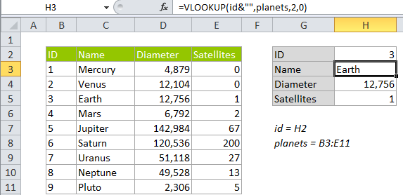
Formula

=VLOOKUP(val&"",table,col,0)

Explanation

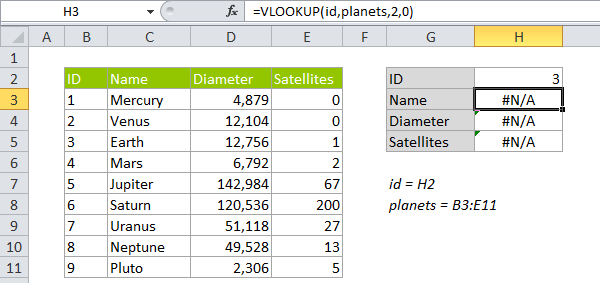
A common problem with VLOOKUP is a mismatch between numbers and text. Either the first column in the table contains lookup values that are numbers stored as text, or the table contains numbers, but the lookup value itself is a number stored as text.

In either case, VLOOKUP will return an #N/A error, even when there appears to be a match. In the example below, each planet has an id based on position from the sun. In cell H3 we have a simple VLOOKUP formula looking for the number 3 from cell H2. The result is the #N/A error, even though 3 is clearly in the table.

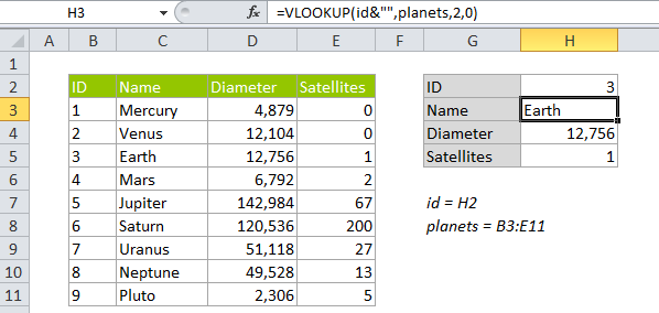
One solution is to convert both the first column in the table and the lookup value to the same type: either numbers or text. However, if you don’t have control over both the table and the lookup value, or if it’s simply not practical to convert values, you can modify the VLOOKUP formula to coerce the lookup value to match the type in the table. In this case, we can revise the VLOOKUP formula to concatenate an empty string to the lookup value, which converts the lookup value to text:

=VLOOKUP(id,planets,2,0)    // original
=VLOOKUP(id&"",planets,2,0) // revised

In the worksheet, the revised formula takes care of the error:

How this formula works

When you concatenate an empty string (“”) to a number, it converts the number to text. You could also do the same thing with a longer formula that utilizes the TEXT function to convert to text :

=VLOOKUP(TEXT(id,"@"),planets,2,0)

If you have both numbers and text

If you can’t be certain when you’ll have numbers and when you’ll have text, you can cater to both options by wrapping VLOOKUP in IFERROR and writing a formula that handles both cases:

=IFERROR(VLOOKUP(id,planets,3,0),VLOOKUP(id&"",planets,3,0))

Here, we first try a straight VLOOKUP formula that assumes both lookup value and the first column in the tables are numbers. If that throws and error, we try again with the revised formula. If that fails, VLOOKUP will return the #N/A error.

Post navigation

Previous Post:

COSH function: Description, Usage, Syntax, Examples and Explanation

Next Post:

Excel Data validation require unique number

Leave a Reply Cancel reply

Your email address will not be published. Required fields are marked *

Learn Basic Excel

Ribbon
Workbook
Worksheets
Format Cells
Find & Select
Sort & Filter
Templates
Print
Share
Protect
Keyboard Shortcuts

Categories

  • Charts
  • Data Analysis
  • Data Validation
  • Excel Functions
    • Cube Functions
    • Database Functions
    • Date and Time Functions
    • Engineering Functions
    • Financial Functions
    • Information Functions
    • Logical Functions
    • Lookup and Reference Functions
    • Math and Trig Functions
    • Statistical Functions
    • Text Functions
    • Web Functions
  • Excel VBA
  • Excel Video Tutorials
  • Formatting
  • Grouping
  • Others

Logical Functions

  • NOT function: Description, Usage, Syntax, Examples and Explanation
  • IF function: Description, Usage, Syntax, Examples and Explanation
  • How to use Excel NOT Function
  • Nested IF function example in Excel
  • How to return blank in place of #DIV/0! error in Excel

Date Time

  • Next biweekly payday from date in Excel
  • Custom weekday abbreviation in Excel
  • Get last working day in month in Excel
  • How to calculate next anniversary date or birthday in Excel
  • Get project end date in Excel

Grouping

  • Map inputs to arbitrary values in Excel
  • Group times into unequal buckets in Excel
  • Categorize text with keywords in Excel
  • How to randomly assign people to groups in Excel
  • Group arbitrary text values in Excel

General

  • Basic text sort formula in Excel
  • Check if multiple cells have same value with case sensitive in Excel
  • Subtotal invoices by age in Excel
  • Customize Ribbon In Excel
  • How to calculate profit margin percentage in Excel
© 2025 xlsoffice . All Right Reserved. | Teal Smiles | Abbreviations And Their Meaning