Skip to content
Free Excel Tutorials
  • Home
  • Excel For Beginners
  • Excel Intermediate
  • Advanced Excel For Experts

Data Analysis

  • Example of COUNTIFS with variable table column in Excel
  • Chart Axes in Excel
  • How To Remove Duplicates In Excel Column Or Row?
  • How to create a Histogram in Excel
  • Everything about Charts in Excel

References

  • Create hyperlink with VLOOKUP in Excel
  • Basic INDEX MATCH approximate in Excel
  • Left Lookup in Excel
  • Vlookup Examples in Excel
  • How to get first column number in range in Excel

Data Validations

  • Excel Data validation allow uppercase only
  • Excel Data validation must begin with
  • Prevent invalid data entering in specific cells
  • Excel Data validation must contain specific text
  • Excel Data validation whole percentage only

VLOOKUP with multiple criteria in Excel

by

This tutorial shows how to calculate VLOOKUP with multiple criteria in Excel using the example below;

Formula

=VLOOKUP(val1&val2,data,column,0)

Explanation

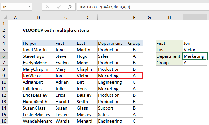
The VLOOKUP function does not handle multiple criteria natively. However, if you have control over source data, you can use a helper column to join multiple fields together, and use these fields like multiple criteria inside VLOOKUP.  In the example shown, Column B is a helper column that concatenates first and last names together, and VLOOKUP does the same to build a lookup value. The formula in I6 is:

=VLOOKUP(I4&I5,data,4,0)

where “data” is the named range B4:F104. The formula in B5 is:

=C5&D5

copied down the table.

How this formula works

In the example shown, we want to lookup employee department and group using VLOOKUP by matching on first and last name.

One limitation of VLOOKUP is that it only handles one condition: the lookup_value, which is matched against the first column in the table. This makes it difficult to use VLOOKUP to find a value based on more than one criteria. However, if you have control over the source data, you an add a helper column that concatenates 2 more more fields together, then give VLOOKUP a lookup value that does the same.

The helper column joins field values from columns that are used as criteria, and it must be the first column of the table. Inside the VLOOKUP function, the lookup value itself is also created by joining the same criteria.

In the example shown, the formula in I6 is:

=VLOOKUP(I4&I5,data,4,0)

Once I4 and I5 are joined, we have:

=VLOOKUP("JonVictor",data,4,0)

VLOOKUP locates “JonVictor” on the 5th row in “data”, and returns the value in the 4th column, “Marketing”.

Setting things up

To set up a multiple criteria VLOOKUP, follow these 3 steps:

  1. Add a helper column and concatenate (join) values from columns you want to use for your criteria.
  2. Set up VLOOKUP to refer to a table that includes the helper column. The helper column must be the first column in the table.
  3. For the lookup value, join the same values in the same order to match values in the helper column.
  4. Make sure VLOOKUP is set to perform an exact match.

Post navigation

Previous Post:

COSH function: Description, Usage, Syntax, Examples and Explanation

Next Post:

Excel Data validation require unique number

Leave a Reply Cancel reply

Your email address will not be published. Required fields are marked *

Learn Basic Excel

Ribbon
Workbook
Worksheets
Format Cells
Find & Select
Sort & Filter
Templates
Print
Share
Protect
Keyboard Shortcuts

Categories

  • Charts
  • Data Analysis
  • Data Validation
  • Excel Functions
    • Cube Functions
    • Database Functions
    • Date and Time Functions
    • Engineering Functions
    • Financial Functions
    • Information Functions
    • Logical Functions
    • Lookup and Reference Functions
    • Math and Trig Functions
    • Statistical Functions
    • Text Functions
    • Web Functions
  • Excel VBA
  • Excel Video Tutorials
  • Formatting
  • Grouping
  • Others

Logical Functions

  • Check multiple cells are equal in Excel
  • Extract multiple matches into separate rows in Excel
  • FALSE function: Description, Usage, Syntax, Examples and Explanation
  • OR function Examples in Excel
  • How to use IFS function in Excel

Date Time

  • Get first day of month in Excel
  • How to calculate workdays per month in Excel
  • Get work hours between dates custom schedule in Excel
  • How to calculate nth day of year in Excel
  • How to calculate quarter from date in Excel

Grouping

  • Map inputs to arbitrary values in Excel
  • Group times into 3 hour buckets in Excel
  • Calculate conditional mode with criteria in Excel
  • Map text to numbers in Excel
  • How to randomly assign people to groups in Excel

General

  • How to calculate percent of goal in Excel
  • Subtotal invoices by age in Excel
  • Check if multiple cells have same value in Excel
  • Flash Fill in Excel
  • Basic text sort formula in Excel
© 2026 xlsoffice . All Right Reserved. | Teal Smiles | Abbreviations And Their Meaning