Skip to content
xlsoffice. All Rights Reserved
  • Home
  • Excel For Beginners
  • Excel Intermediate
  • Advanced Excel For Experts

Lookup and Reference Examples

  • INDEX function: Description, Usage, Syntax, Examples and Explanation
  • How to get relative row numbers in a range in Excel
  • How to use Excel INDIRECT Function
  • Extract all partial matches in Excel
  • How to calculate two-way lookup VLOOKUP in Excel Table

Data Analysis Examples

  • How To Filter Data in Excel
  • Filter Data Based on Date in Excel
  • How to calculate current stock or inventory in Excel
  • How to calculate correlation coefficient Correlation in Excel
  • Get column name from index in Excel Table

Data Validation Examples

  • Excel Data validation no punctuation
  • Excel Data validation must begin with
  • Excel Data validation must not contain
  • Excel Data validation must contain specific text
  • Excel Data validation unique values only

Sum top n values in Excel

by

This tutorial shows how to Sum top n values in Excel using the example below;

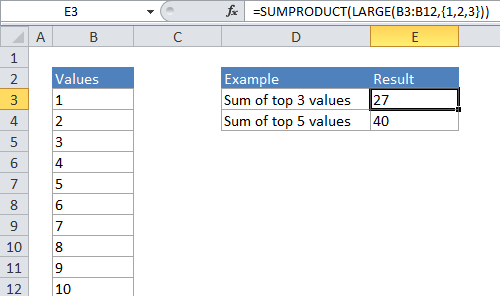
To sum the top values in a range, you can use a formula based on the LARGE function, wrapped inside the SUMPRODUCT function.

Formula

=SUMPRODUCT(LARGE(range,{1,2,N}))

Explanation

In the generic form of the formula (above), a range of cells that contain numeric values and N represents the idea of Nth value.

In the example, the active cell contains this formula:

=SUMPRODUCT(LARGE(B4:B13,{1,2,3}))

How this formula works

In its simplest form, LARGE will return the “Nth largest” value in a range. For example, the formula:

=LARGE(B4:B13, 2)

will return the 2nd largest value in the range B4:B13 which, in the example above, is the number 9.

Worked Example:   Count total matches in two ranges in Excel

However, if you supply an “array constant” (e.g. a constant in the form {1,2,3}) to LARGE as the second argument, LARGE will return an array of results instead of a single result. So, the formula:

=LARGE(B4:B13,{1,2,3})

will return the 1st, 2nd, and 3rd largest value in the range B4:B13. In the example above, where B4:B13 contains the numbers 1-10, the result from LARGE will be the array {8,9,10}. SUMPRODUCT then sums the numbers in this array and returns a total, which is 27.

Worked Example:   Highlight duplicate rows in Excel

SUM instead of SUMPRODUCT

SUMPRODUCT is a flexible function that allows you to uses cell references for k inside the LARGE function.

However, if you are using a simple hard-coded array constant like {1,2,3} you can just use the SUM function:

=SUM(LARGE(B4:B13,{1,2,3}))

Note you must enter this formula as an array formula if you use cell references and not an array constant for k inside LARGE.

When N becomes large

When N becomes large it becomes tedious to create the array constant by hand – If you want to sum to the top 20 or 30 values in a large list, typing out an array constant with 20 or 30 items will take a long time. In this case, you can use a shortcut for building the array constant that uses the ROW and INDIRECT functions.

Worked Example:   How to check cell equals one of many things in Excel

For example, if you want to SUM the top 20 values in a range called “rng” you can write a formula like this:

=SUMPRODUCT(LARGE(rng,ROW(INDIRECT("1:20"))))

Variable N

With insufficient data, a fixed N can cause errors. In this case, you can try a formula like this:

=SUMPRODUCT(LARGE(rng,ROW(INDIRECT("1:"&MIN(3,COUNT(rng))))))

Here, we use MIN with COUNT to sum the top 3 values, or the count of values, if less than 3.

Post navigation

Previous Post:

SUMPRODUCT with IF in Excel

Next Post:

Sum visible rows in a filtered list in Excel

Leave a Reply Cancel reply

Your email address will not be published. Required fields are marked *

Learn Basic Excel

Ribbon
Workbook
Worksheets
Format Cells
Find & Select
Sort & Filter
Templates
Print
Share
Protect
Keyboard Shortcuts

Categories

  • Charts
  • Data Analysis
  • Data Validation
  • Excel Functions
    • Cube Functions
    • Database Functions
    • Date and Time Functions
    • Engineering Functions
    • Financial Functions
    • Information Functions
    • Logical Functions
    • Lookup and Reference Functions
    • Math and Trig Functions
    • Statistical Functions
    • Text Functions
    • Web Functions
  • Excel VBA
  • Excel Video Tutorials
  • Formatting
  • Grouping
  • Others
  • LOWER function: Description, Usage, Syntax, Examples and Explanation
  • FIND, FINDB functions: Description, Usage, Syntax, Examples and Explanation
  • How to count specific words in a range in Excel
  • CHAR function: Description, Usage, Syntax, Examples and Explanation
  • Count Number of Words in Excel
  • Custom weekday abbreviation in Excel
  • HOUR function: Description, Usage, Syntax, Examples and Explanation
  • Calculate series of dates by workdays in Excel
  • Calculate expiration date in Excel
  • How to get same date next year or previous year in Excel
  • COUPDAYSNC function: Description, Usage, Syntax, Examples and Explanation
  • TBILLPRICE function: Description, Usage, Syntax, Examples and Explanation
  • PRICEDISC function: Description, Usage, Syntax, Examples and Explanation
  • ODDLYIELD function: Description, Usage, Syntax, Examples and Explanation
  • DOLLARFR function: Description, Usage, Syntax, Examples and Explanation
Acronyms, Abbreviations, Initialism & What They Stand For
© 2022 xlsoffice . All Right Reserved. | Teal Smiles