Skip to content
Free Excel Tutorials
  • Home
  • Excel For Beginners
  • Excel Intermediate
  • Advanced Excel For Experts

Data Analysis

  • How to Sort by Color in Excel
  • Number and Text Filters Examples in Excel
  • Excel Frequency Function Example
  • How to create running total in an Excel Table
  • Get column index in Excel Table

References

  • Last row number in range
  • How to retrieve first match between two ranges in Excel
  • How to calculate two-way lookup VLOOKUP in Excel Table
  • Basic INDEX MATCH approximate in Excel
  • How to use Excel ROWS Function

Data Validations

  • How To Create Drop-down List in Excel
  • Excel Data validation allow weekday only
  • Excel Data validation must contain specific text
  • Excel Data validation whole percentage only
  • Excel Data validation date in next 30 days

Sum if cells contain either x or y in Excel

by

This tutorial shows how to Sum if cells contain either x or y in Excel using the example below;
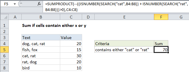
Formula

=SUMPRODUCT(--((ISNUMBER(SEARCH("cat",range1)) + ISNUMBER(SEARCH("rat",range1)))>0),range2)

Explanation

To sum if cells contain either one text string or another (i.e. contain “cat” or “rat”) you can use the SUMPRODUCT function.

Background

When you sum cells with “OR” criteria, you need to be careful not to double count when there is a possibility that both criteria will return true. In the example shown, we want to sum values in Column C when cells in column B contain either “cat” or “rat”. We can’t use SUMIFs with two criteria, because SUMIFS is based on AND logic. And if we try to use two SUMIFS (i.e. SUMIFS + SUMIFS) we will double count because there are cells that contain both “cat” and “rat”

Solution

One solution is to use  SUMPRODUCT with ISNUMBER + SEARCH or FIND. The formula in cell F4 is:

=SUMPRODUCT(--((ISNUMBER(SEARCH("cat",B4:B8)) + ISNUMBER(SEARCH("rat",B4:B8)))>0),C4:C8)

This formula is based the formula here that locates text inside of a cell:

ISNUMBER(SEARCH("abc",B4:B10)

When given a range of cells, this snippet will return an array of TRUE/FALSE values, one value for each cell the range. Since we are using this twice (once for “cat” and once for “rat”), we’ll get two arrays.

Next, we add these arrays together (with +), which creates a new single array of numbers. Each number in this array is the result of adding the TRUE and FALSE values in the original two arrays together. In the example shown, the array looks like this:

{2;0;2;1;0}

We need to add these numbers up, but we don’t want to double count. So we need to make sure any value greater than zero is just counted once. To do that, we force all values to TRUE or FALSE by checking the array with “>0”. This returns TRUE / FALSE:

{TRUE;FALSE;TRUE;TRUE;FALSE}

Which we then convert to 1 / 0 using a double negative (–):

{1;0;1;1;0}

Case-sensitive option

The SEARCH function ignores case. If you need a sensitive option, replace SEARCH with FIND.

Post navigation

Previous Post:

How to use Excel CHOOSE Function

Next Post:

Customize Ribbon In Excel

Leave a Reply Cancel reply

Your email address will not be published. Required fields are marked *

Learn Basic Excel

Ribbon
Workbook
Worksheets
Format Cells
Find & Select
Sort & Filter
Templates
Print
Share
Protect
Keyboard Shortcuts

Categories

  • Charts
  • Data Analysis
  • Data Validation
  • Excel Functions
    • Cube Functions
    • Database Functions
    • Date and Time Functions
    • Engineering Functions
    • Financial Functions
    • Information Functions
    • Logical Functions
    • Lookup and Reference Functions
    • Math and Trig Functions
    • Statistical Functions
    • Text Functions
    • Web Functions
  • Excel VBA
  • Excel Video Tutorials
  • Formatting
  • Grouping
  • Others

Logical Functions

  • NOT function: Description, Usage, Syntax, Examples and Explanation
  • SWITCH function example in Excel
  • SWITCH function: Description, Usage, Syntax, Examples and Explanation
  • IF function: Description, Usage, Syntax, Examples and Explanation
  • IFERROR function: Description, Usage, Syntax, Examples and Explanation

Date Time

  • How to show last updated date stamp in Excel
  • Two ways to sum time over 30 minutes in Excel
  • Get date from day number in Excel
  • Get last weekday in month in Excel
  • Convert decimal minutes to Excel time

Grouping

  • Group times into unequal buckets in Excel
  • Group numbers at uneven intervals in Excel
  • Calculate conditional mode with criteria in Excel
  • If cell contains one of many things in Excel
  • Map text to numbers in Excel

General

  • Subtotal by invoice number in Excel
  • Print Excel Sheet In Landscape Or Portrait
  • How to fill cell ranges with random number from fixed set of options in Excel
  • Mark Workbook as Final in Excel
  • Freeze and Unfreeze Panes in Excel
© 2025 xlsoffice . All Right Reserved. | Teal Smiles | Abbreviations And Their Meaning