INDEX and MATCH with multiple criteria in Excel

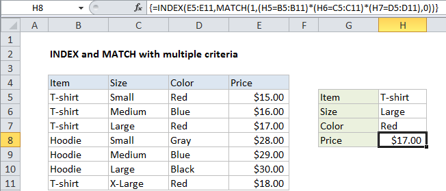
To lookup values with INDEX and MATCH, using multiple criteria, you can use an array formula. In the example shown, the formula in H8 is:

{=INDEX(E5:E11,MATCH(1,(H5=B5:B11)*(H6=C5:C11)*(H7=D5:D11),0))}

Note: this is an array formula, and must be entered with control + shift + enter.

How this formula works

Normally, and INDEX MATCH formula is configured with MATCH set to look through a one-column range and provide a match based on a given criteria. Without concatenating values in a helper column, or in the formula itself, there’s no way to supply more than one criteria.

This formula works around this limitation by using boolean logic to create an array of ones and zeros to represent rows matching all 3 criteria, then using MATCH to match the first 1 found.

The temporary array of ones and zeros is based on this snippet:

(H5=B5:B11)*(H6=C5:C11)*(H7=D5:D11)

Here we compare the item H5 against all items, the size in H6 against all sizes, and the color in H7 against all colors. the initial result looks like this:

{TRUE;TRUE;TRUE;FALSE;FALSE;FALSE;TRUE}*{FALSE;FALSE;TRUE;FALSE;FALSE;TRUE;FALSE}*{TRUE;FALSE;TRUE;FALSE;FALSE;FALSE;TRUE}

The multiplication operation transforms the TRUE FALSE values to 1s and 0s:

{1;1;1;0;0;0;1}*{0;0;1;0;0;1;0}*{1;0;1;0;0;0;1}

And the final result looks like this:

{0;0;1;0;0;0;0}

Which goes into MATCH as the lookup array:

MATCH(1,{0;0;1;0;0;0;0})

MATCH returns 3, and the entire formula boils down to a standard INDEX MATCH formula

=INDEX(E5:E11,3)

with a final result of $17.00.

Non-array version

It is possible to add another INDEX to this formula, avoiding the need to enter as an array formula with control + shift + enter:

=INDEX(rng1,MATCH(1,INDEX((A1=rng2)*(B1=rng3)*(C1=rng4),0,1),0))

The INDEX function can handle arrays natively, so the second INDEX is added only to “catch” the array created with the boolean logic operation and return the same array again to MATCH. To do this, INDEX is configured with zero rows and one column. The zero row trick causes INDEX to return column 1 from the array (which is already one column anyway).