How to import data into Excel using Microsoft Query Wizard

This example teaches you how to import data from a Microsoft Access database by using the Microsoft Query Wizard. With Microsoft Query, you can select the columns of data that you want and import only that data into Excel.

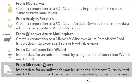
1. On the Data tab, in the Get External Data group, click From Other Sources.

2. Click From Microsoft Query.

The ‘Choose Data Source” dialog box appears.

3. Select MS Access Database* and check ‘Use the Query Wizard to create/edit queries’.

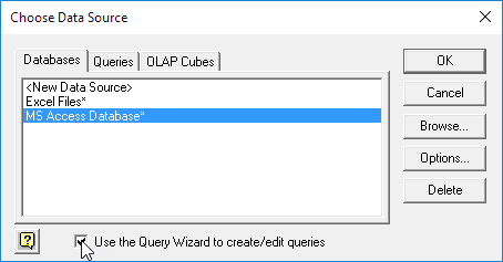
4. Click OK.

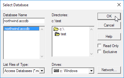
5. Select the database and click OK.

This Access database consists of multiple tables. You can select the table and columns you want to include in your query.

6. Select Customers and click the > symbol.

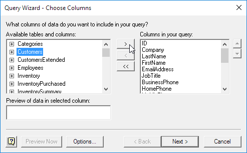
7. Click Next.

To only import a specified set of records, filter the data.

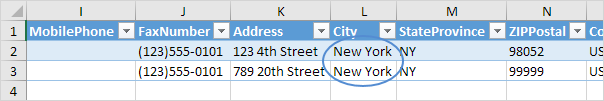
8. Click City from the ‘Column to filter’ list and only include rows where City equals New York.

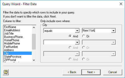
9. Click Next.

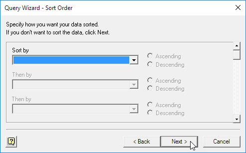
You can sort your data if you want (we don’t do it here).

10. Click Next.

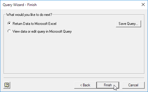
11. Click Finish to return the data to Microsoft Excel.

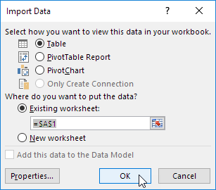
12. Select how you want to view this data, where you want to put it, and click OK.

Result:

13. When your Access data changes, you can easily refresh the data in Excel. First, select a cell inside the table. Next, on the Design tab, in the External Table Data group, click Refresh.