Get first match cell contains in Excel

This tutorial shows how to Get first match cell contains in Excel using the example below;

Formula

{=INDEX(things,MATCH(TRUE,ISNUMBER(SEARCH(things,A1)),0))}

Explanation

To check a cell for one of several things, and return the first match found in the list, you can use an INDEX / MATCH formula that uses SEARCH or FIND to locate a match.

This is an array formula and must be entered with Control + Shift + Enter.

Context

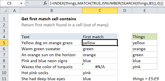
You have a list of things in the range B5:B11, and you want to check cells to see if they contain any of these things. If so, you want the first match found.

Solution

To find partial matches inside a cell, you can use a formula based on SEARCH (not case-sensitive) or FIND (case-sensitive). This formula needs to be adapted to look for multiple values in the same cell.

The final solution uses the MATCH function to figure out the first item that matches in the list of things, and the the INDEX function to retrieve the actual match. In the example shown, the formula in C5 is:

{=INDEX(things,MATCH(TRUE,ISNUMBER(SEARCH(things,B5)),0))}

How this formula works

The core of this formula is this snippet:

ISNUMBER(SEARCH(things,B5)

This is based on another formula (explained in detail here) that checks a cell for a single substring. If the cell contains the substring, the formula returns TRUE. If not, the formula returns FALSE.

When we give this SEARCH a list of things (instead of one thing) will give us back a list of positions. The ISNUMBER function then translates these positions to TRUE / FALSE values. Any valid number becomes TRUE, and any error (not found) becomes FALSE. The result is an array like this:

{TRUE;TRUE;FALSE;FALSE;FALSE}

MATCH then gets the position of the first match, by looking for TRUE.

INDEX uses this position as the row number, with “things” as the array to fetch an item from the list of things. When no match is found, this formula returns #N/A.

With hard-coded values

If you don’t want to set up an external named range like “things” in this example, you can hard-code values into the formula as “array constants” like this:

{=INDEX({"red","green","blue"},MATCH(TRUE,ISNUMBER(SEARCH({"red","green","blue"},B5)),0))}