Find missing values in Excel

=IF(COUNTIF(list,value),"OK","Missing")

If you want to find out what values in one list are missing from another list, you can use a  simple formula based on the COUNTIF function.

The COUNTIF function counts cells that meet supplied criteria, returning the number of occurrences found. If no cells that meet criteria are found, COUNTIF returns zero. You can use behavior directly inside an IF statement to identify values that have a zero count (i.e. values that are missing).

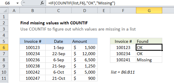
In the example shown, the formula in G6 is:

=IF(COUNTIF(list,F6),"OK","Missing")

where “list” is a named range that corresponds to the range B6:B11.

The IF function requires a logical test to return TRUE or FALSE. In this case, if a value is found, a positive number is returned by COUNTIF, which evaluates to TRUE, causing IF to return “OK”. If no value is found, zero is returned, which evaluates to FALSE, and IF returns “Missing”.

Alternative with MATCH

You can also test for missing values using the MATCH function. MATCH finds the position of an item in a list and will return the #N/A error when a value is not found. You can use this behavior to build a formula that returns “Missing” or “OK” by testting the result of MATCH using another function called ISNA. ISNA returns true only when it receives the #N/A error.

To use MATCH as shown in the example above, the formula is:

=IF(ISNA(MATCH(F6,list,0)),"Missing","OK")