Find longest string in column in Excel

{=INDEX(range,MATCH(MAX(LEN(range)),LEN(range),0))}

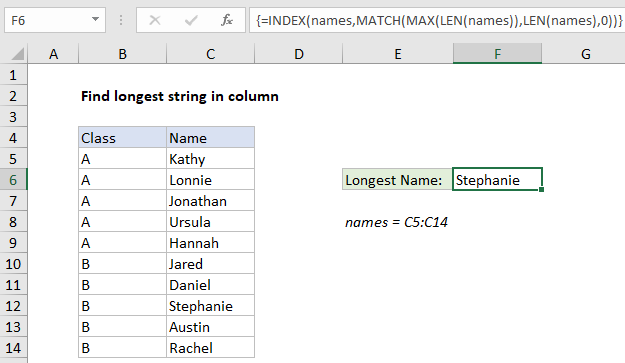
To find the longest string (name, word, etc.) in a column, you can use an array formula based on INDEX and MATCH, together with LEN and MAX. In the example shown, the formula in F6 is:

{=INDEX(names,MATCH(MAX(LEN(names)),LEN(names),0))}

Where “names” is the named range C5:C14.

Note: this is an array formula and must be entered with control + shift + enter.

How this formula works

The key to this formula is the MATCH function, which is set up like this:

MATCH(MAX(LEN(name)),LEN(name),0))

In this snippet, MATCH is set up to perform an exact match by supplying zero for match type. For lookup value, we have this:

MAX(LEN(names))

Here, the LEN function returns an array of results (lengths), one for each name in the list:

{5;6;8;6;6;5;6;9;6;6}

The MAX function then returns the largest value, 9 in this case. For lookup array, LEN is again used to return an array of lengths. The after LEN and MAX run, we have:

MATCH(9,{5;6;8;6;6;5;6;9;6;6},0)

which returns the position of the max value, 8.

This goes into INDEX like this:

=INDEX(names,8)

INDEX duly returns the value in the 8th position of names,  which is “Stephanie”.