Skip to content
xlsoffice. All Rights Reserved
  • Home
  • Excel For Beginners
  • Excel Intermediate
  • Advanced Excel For Experts

Lookup and Reference Examples

  • How to get address of first cell in range in Excel
  • Get nth match with INDEX / MATCH in Excel
  • How to get first column number in range in Excel
  • To count total rows in a range in Excel
  • How to reference named range different sheet in Excel

Data Analysis Examples

  • How to add Trendline to a chart in Excel
  • Working With Tables in Excel
  • How To Insert and Customize Sparklines in Excel
  • How to perform a t-Test in Excel
  • Add Outline to Data in Excel

Data Validation Examples

  • Excel Data validation allow uppercase only
  • Excel Data validation unique values only
  • Excel Data validation whole percentage only
  • Excel Data validation number multiple 100
  • Excel Data validation no punctuation

Excel Data validation allow numbers only

by

This tutorial shows how to create Data validation to allow numbers only in Excel using the example below;

Formula

=ISNUMBER(A1)

Explanation

Note: Excel has several built-in data validation rules for numbers. This page explains how to create a your own validation rule based on a custom formula.

Worked Example:   IS functions: ISBLANK, ISERR, ISERROR, ISLOGICAL, ISNA, ISNONTEXT, ISNUMBER, ISREF, ISTEXT

To allow only numbers in a cell, you can use data validation with a custom formula based on the ISNUMBER function.

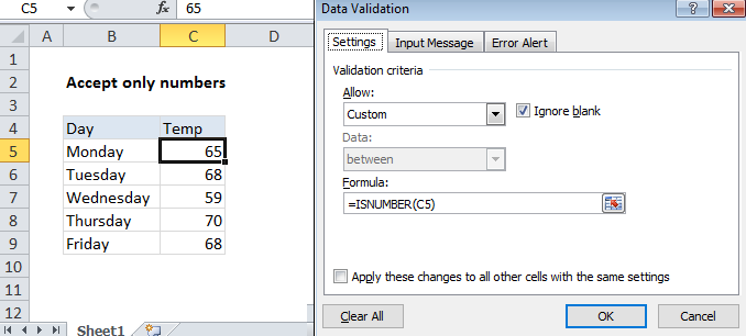
In the example shown, the data validation applied to C5:C9 is:

=ISNUMBER(C5)

How this formula works

Data validation rules are triggered when a user adds or changes a cell value.

Worked Example:   If cell contains in Excel

The ISNUMBER function returns TRUE when a value is numeric and FALSE if not. As a result, all numeric input will pass validation.

Be aware that numeric input includes dates and times, whole numbers, and decimal values.

Worked Example:   Highlight cells that contain one of many in Excel

Note:  Cell references in data validation formulas are relative to the upper left cell in the range selected when the validation rule is defined, in this case C5.

Post navigation

Previous Post:

Highlight dates in same month and year in Excel

Next Post:

Excel Data validation allow text only

Leave a Reply Cancel reply

Your email address will not be published. Required fields are marked *

Learn Basic Excel

Ribbon
Workbook
Worksheets
Format Cells
Find & Select
Sort & Filter
Templates
Print
Share
Protect
Keyboard Shortcuts

Categories

  • Charts
  • Data Analysis
  • Data Validation
  • Excel Functions
    • Cube Functions
    • Database Functions
    • Date and Time Functions
    • Engineering Functions
    • Financial Functions
    • Information Functions
    • Logical Functions
    • Lookup and Reference Functions
    • Math and Trig Functions
    • Statistical Functions
    • Text Functions
    • Web Functions
  • Excel VBA
  • Excel Video Tutorials
  • Formatting
  • Grouping
  • Others
  • Clean and reformat telephone numbers using SUBSTITUTE function in Excel
  • Complete List of Excel Text Functions References and Examples
  • Replace one character with another in Excel
  • Get first name from full name — Manipulating NAMES in Excel
  • CODE function: Description, Usage, Syntax, Examples and Explanation
  • How to calculate quarter from date in Excel
  • Get days before a date in Excel
  • Two ways to sum time over 30 minutes in Excel
  • How to get same date next year or previous year in Excel
  • EOMONTH function: Description, Usage, Syntax, Examples and Explanation
  • FV function: Description, Usage, Syntax, Examples and Explanation
  • RATE function: Description, Usage, Syntax, Examples and Explanation
  • PRICEDISC function: Description, Usage, Syntax, Examples and Explanation
  • ODDFYIELD function: Description, Usage, Syntax, Examples and Explanation
  • TBILLEQ function: Description, Usage, Syntax, Examples and Explanation
© 2022 xlsoffice . All Right Reserved. | Teal Smiles