
Skip to content
Free Excel Tutorials
  • Home
  • Excel For Beginners
  • Excel Intermediate
  • Advanced Excel For Experts

Data Analysis

  • How To Insert and Customize Sparklines in Excel
  • Filter Data Based on Date in Excel
  • Conditional Formatting New Rule with Formulas in Excel
  • Conditional Formatting Color Scales Examples in Excel
  • Randomize/ Shuffle List in Excel

References

  • Convert text string to valid reference in Excel using Indirect function
  • How to retrieve first match between two ranges in Excel
  • How to use Excel FORMULATEXT function
  • Basic INDEX MATCH approximate in Excel
  • How to use Excel LOOKUP Function

Data Validations

  • Excel Data validation exists in list
  • Excel Data validation must begin with
  • Excel Data validation must contain specific text
  • Excel Data validation whole percentage only
  • Excel Data validation unique values only

Split dimensions into three parts in Excel

by

To split dimensions that like 100x50x25 into three separate parts, you can use some rather complicated formulas that use LEFT, MID, RIGHT, FIND, LEN, and SUBSTITUTE.

Note: you can also use Flash Fill in Excel 2013 and above, and the “text to columns” feature in older versions of Excel. Both approaches are quite a bit simpler than the formulas described below. However, if you need a dynamic solution, read on…

Formula

=LEFT(B4,FIND("x",B4)-1)
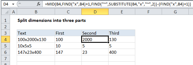
Explanation


The 1st dimension

To get the first dimension, we are using this formula in C4:

=LEFT(B4,FIND("x",B4)-1)

This works by extracting text starting at the LEFT. The number of characters is calculated by locating the first “x” in the text using the FIND function, then subtracting 1.

The 2nd dimension

To get the second dimension, we are using this formula in D4:

=MID(B4,FIND("x",B4)+1,FIND("~",SUBSTITUTE(B4,"x","~",2))-(FIND("x",B4)+1))

This formula uses the MID function, which extracts a certain number of characters starting at a certain position in the next. The starting position is calculated with this:

FIND("x",B4)+1

Which simply locates the first “x” and adds 1.

The number of characters is calculated using:

FIND("~",SUBSTITUTE(B4,"x","~",2))-(FIND("x",B4)+1)

We use SUBSTITUTE with FIND to locate the position of the 2nd “x”, as described here.

We then subtract from that the location of the first “x” + 1.

The 3rd dimension

To get the third dimension, we are using this formula in E4:

=RIGHT(B4,LEN(B4)-FIND("~",SUBSTITUTE(B4,"x","~",2)))

This uses the RIGHT function to extract a specific number of characters, starting from the right. We calculate the number of characters to extract by getting the total length with LEN, then subtracting the location of the 2nd instance of “x”.

Post navigation

Next Post:

Create One-dimensional and Two-dimensional Array

Leave a Reply Cancel reply

Your email address will not be published. Required fields are marked *

Learn Basic Excel

Ribbon
Workbook
Worksheets
Format Cells
Find & Select
Sort & Filter
Templates
Print
Share
Protect
Keyboard Shortcuts

Categories

  • Charts
  • Data Analysis
  • Data Validation
  • Excel Functions
    • Cube Functions
    • Database Functions
    • Date and Time Functions
    • Engineering Functions
    • Financial Functions
    • Information Functions
    • Logical Functions
    • Lookup and Reference Functions
    • Math and Trig Functions
    • Statistical Functions
    • Text Functions
    • Web Functions
  • Excel VBA
  • Excel Video Tutorials
  • Formatting
  • Grouping
  • Others

Logical Functions

  • IF with wildcards in Excel
  • How to use Excel NOT Function
  • AND function: Description, Usage, Syntax, Examples and Explanation
  • Check multiple cells are equal in Excel
  • Extract multiple matches into separate rows in Excel

Date Time

  • Add decimal hours to time in Excel
  • Calculate date overlap in days in Excel
  • Add business days to date in Excel
  • Roll back weekday to Friday base on a particular date in Excel
  • How to calculate quarter from date in Excel

Grouping

  • How to randomly assign people to groups in Excel
  • Calculate conditional mode with criteria in Excel
  • Group numbers with VLOOKUP in Excel
  • How to randomly assign data to groups in Excel
  • Running count group by n size in Excel

General

  • How to calculate profit margin percentage in Excel
  • How to create dynamic worksheet reference in Excel
  • Subtotal by color in Excel
  • Check if multiple cells have same value in Excel
  • Spell Check in Excel
© 2026 xlsoffice . All Right Reserved. | Teal Smiles | Abbreviations And Their Meaning