Skip to content
Free Excel Tutorials
  • Home
  • Excel For Beginners
  • Excel Intermediate
  • Advanced Excel For Experts

Data Analysis

  • Number and Text Filters Examples in Excel
  • How to Create One and Two Variable Data Tables in Excel
  • Conditional Formatting New Rule with Formulas in Excel
  • How to create a Histogram in Excel
  • How To Insert and Customize Sparklines in Excel

References

  • Find Closest Match in Excel Using INDEX, MATCH, ABS and MIN functions
  • Extract all partial matches in Excel
  • Excel Advanced Lookup using Index and Match Functions
  • CHOOSE function: Description, Usage, Syntax, Examples and Explanation
  • Lookup entire row in Excel

Data Validations

  • Prevent invalid data entering in specific cells
  • Data validation must not exist in list
  • Excel Data validation exists in list
  • Excel Data validation must not contain
  • Excel Data validation unique values only

How to find nth occurrence of character in Excel

by

To find the nth occurrence of a character in a text string, you can use a formula based on the FIND and SUBSTITUTE functions.

Formula

=FIND(CHAR(160),SUBSTITUTE
(text,"@",CHAR(160),N))

Explanation

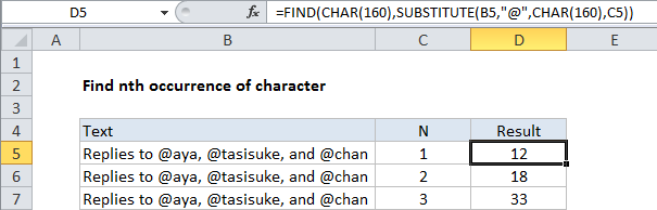
In the example shown, the formula in D5 is:

=FIND(CHAR(160),SUBSTITUTE
(B5,"@",CHAR(160),C5))

How this formula works

In this example we are looking for the nth occurrence of the “@” character.

Working from the inside out, we first use the SUBSTITUTE function to replace the nth occurrence of “@” with CHAR(160):

SUBSTITUTE(B5,"@",CHAR(160),C5)

The SUBSTITUTE function has an optional 4th argument called instance number that can be used to specify the instance that should be replaced. This number comes from column C.

SUBSTITUTE then replaces the nth occurrence of “@” with CHAR(160), which resolves to “†”. We use CHAR(160) because it won’t normally appear in text. You can use any character you know won’t exist in the text.

Finally, the FIND character looks for CHAR(160) and returns the position.

Post navigation

Next Post:

Create One-dimensional and Two-dimensional Array

Leave a Reply Cancel reply

Your email address will not be published. Required fields are marked *

Learn Basic Excel

Ribbon
Workbook
Worksheets
Format Cells
Find & Select
Sort & Filter
Templates
Print
Share
Protect
Keyboard Shortcuts

Categories

  • Charts
  • Data Analysis
  • Data Validation
  • Excel Functions
    • Cube Functions
    • Database Functions
    • Date and Time Functions
    • Engineering Functions
    • Financial Functions
    • Information Functions
    • Logical Functions
    • Lookup and Reference Functions
    • Math and Trig Functions
    • Statistical Functions
    • Text Functions
    • Web Functions
  • Excel VBA
  • Excel Video Tutorials
  • Formatting
  • Grouping
  • Others

Logical Functions

  • Complete List of Excel Logical Functions, References and Examples
  • Invoice status with nested if in Excel
  • How to return blank in place of #DIV/0! error in Excel
  • XOR function: Description, Usage, Syntax, Examples and Explanation
  • SWITCH function: Description, Usage, Syntax, Examples and Explanation

Date Time

  • How to calculate workdays per month in Excel
  • Get day from date in Excel
  • Convert date to text in Excel
  • Display Date is workday in Excel
  • Add decimal minutes to time in Excel

Grouping

  • Calculate conditional mode with criteria in Excel
  • Group times into unequal buckets in Excel
  • Group numbers with VLOOKUP in Excel
  • Map text to numbers in Excel
  • Categorize text with keywords in Excel

General

  • How to count total columns in range in Excel
  • How to create dynamic worksheet reference in Excel
  • How to get random value from list or table in Excel
  • How to generate random number between two numbers in Excel
  • Transpose: Switch ‘Rows to Columns’ or ‘Columns to Rows’ in Excel
© 2026 xlsoffice . All Right Reserved. | Teal Smiles | Abbreviations And Their Meaning