How to find and replace multiple values at same time in Excel

To find and replace multiple values with a formula, you can nest multiple SUBSTITUTE functions together, and feed in find/replace pairs from another table using the INDEX function.

Formula

=SUBSTITUTE(SUBSTITUTE(B5,INDEX(find,1),INDEX(replace,1)),
INDEX(find,2),INDEX(replace,2))

Explanation

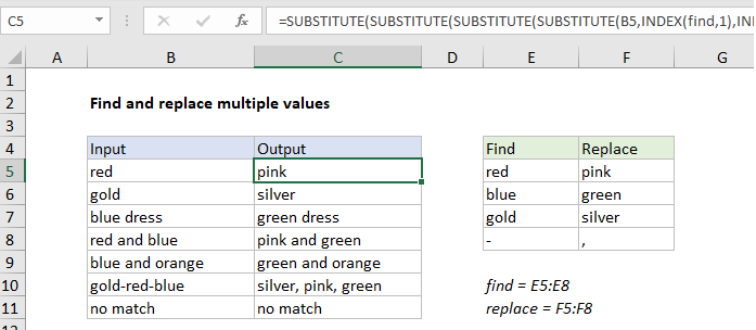
In the example shown, we are performing 4 separate find and replace operations. The formula in G5 is:

=SUBSTITUTE(SUBSTITUTE(SUBSTITUTE(SUBSTITUTE(B5,INDEX(find,1),
INDEX(replace,1)),INDEX(find,2),INDEX(replace,2)),
INDEX(find,3),INDEX(replace,3)),INDEX(find,4),INDEX(replace,4))

where “find” is the named range E5:E8, and “replace” is the named range F5:F8. See below for info on how to make this formula easier to read.

Preface

There is no built-in formula for running a series of find and replace operations in Excel, so this a “concept” formula to show one approach. The text to look for and replace with is stored directly on the worksheet in a table, and retrieved with the INDEX function. This makes the solution “dynamic” – any of these values are changed, results update immediately. Of course, there is no requirement to use INDEX; you can hard-code values into the formula if you prefer.

How this formula works

At the core, the formula uses the SUBSTITUTE function to perform the each substitution, with this basic pattern:

=SUBSTITUTE(text,find,replace)

“Text” is the incoming value, “find” is the text to look for, and “replace” is the text to replace with. The text to look for and replace with is stored in the table to the right, in the range E5:F8, one pair per row. The values on the left are in the named range”find”and the values on the right are in the named range “replace”.  The INDEX function is used to retrieve both the “find” text and the “replace” text like this:

INDEX(find,1) // first "find" value
INDEX(replace,1) // first "replace" value

So, to run the first substitution (look for “red”, replace with “pink”) we use:

=SUBSTITUTE(B5,INDEX(find,1),INDEX(replace,1))

In total, we run four separate substitutions, and each subsequent SUBSTITUTE begins with the result from the previous SUBSTITUTE:

=SUBSTITUTE(SUBSTITUTE(SUBSTITUTE(SUBSTITUTE(B5,INDEX(find,1),
INDEX(replace,1)),INDEX(find,2),INDEX(replace,2)),
INDEX(find,3),INDEX(replace,3)),INDEX(find,4),INDEX(replace,4))

Line breaks for readability

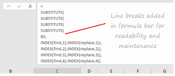
You’ll notice this kind of nested formula is quite difficult to read. By adding line breaks, we can make the formula much easier to read and maintain:

=
SUBSTITUTE(
SUBSTITUTE(
SUBSTITUTE(
SUBSTITUTE(
B5,
INDEX(find,1),INDEX(replace,1)),
INDEX(find,2),INDEX(replace,2)),
INDEX(find,3),INDEX(replace,3)),
INDEX(find,4),INDEX(replace,4))

The formula bar in Excel ignores extra white space and line breaks, so the above formula can be pasted in directly:

By the way, there is a keyboard shortcut for expanding and collapsing the formula bar.

More substitutions

More rows can be added to the table to handle more find/replace pairs. Each time a pair is added, the formula needs to be updated to include the new pair. It’s important also to make sure the named ranges (if you are using them) are updated to include new values as needed. Alternately, you could use a proper Excel Table for dynamic ranges, instead of named ranges.

Other uses

The same approach can be used clean up text by “stripping” punctuation and other symbols from text with a series of substitutions.