Skip to content
Free Excel Tutorials
  • Home
  • Excel For Beginners
  • Excel Intermediate
  • Advanced Excel For Experts

Data Analysis

  • What-If Analysis: Scenarios and Goal Seek in Excel
  • Conflicting Multiple Conditional Formatting Rules in Excel
  • How To Create Pareto Chart in Excel
  • How to create Checklist in Excel
  • How to do a t-Test in Excel?

References

  • How to get last column number in range in Excel
  • How to get first row number in range in Excel
  • LOOKUP function: Description, Usage, Syntax, Examples and Explanation
  • Count rows that contain specific values in Excel
  • How to get address of last cell in range in Excel

Data Validations

  • Excel Data validation must contain specific text
  • Excel Data validation don’t exceed total
  • Excel Data validation allow uppercase only
  • Excel Data validation require unique number
  • Excel Data validation whole percentage only

How to count specific characters in a cell in Excel

by

To count how many times a specific character appears in a cell, you can use a formula based on the SUBSTITUTE and LEN functions.

Formula

=LEN(A1)-LEN(SUBSTITUTE(A1,"a",""))

Explanation


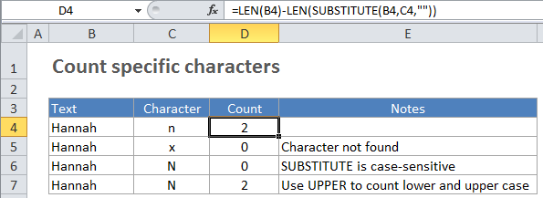
In the example, the active cell contains this formula:

=LEN(B3)-LEN(SUBSTITUTE(B3,C3,""))

How this formula works

This formula works by using SUBSTITUTE to first remove all of the characters being counted in the source text. Then the length of the text (with the character removed) is subtracted from the length of the original text. The result is the number of characters that were removed with SUBSTITUTE, which is equal to the count of those characters.

Upper and lower case

SUBSTITUTE is a case sensitive function, so it will match case when running a substitution. If you need to count both upper and lower case occurrences of a specific character, use the UPPER function inside SUBSTITUTE to convert the text to uppercase before running the substitution. Then supply an uppercase character as the text that’s being substituted like this:

=LEN(A1)-LEN(SUBSTITUTE(UPPER(A1),"A",""))

Post navigation

Next Post:

Create One-dimensional and Two-dimensional Array

Leave a Reply Cancel reply

Your email address will not be published. Required fields are marked *

Learn Basic Excel

Ribbon
Workbook
Worksheets
Format Cells
Find & Select
Sort & Filter
Templates
Print
Share
Protect
Keyboard Shortcuts

Categories

  • Charts
  • Data Analysis
  • Data Validation
  • Excel Functions
    • Cube Functions
    • Database Functions
    • Date and Time Functions
    • Engineering Functions
    • Financial Functions
    • Information Functions
    • Logical Functions
    • Lookup and Reference Functions
    • Math and Trig Functions
    • Statistical Functions
    • Text Functions
    • Web Functions
  • Excel VBA
  • Excel Video Tutorials
  • Formatting
  • Grouping
  • Others

Logical Functions

  • How to use Excel TRUE Function
  • Return blank if in Excel
  • How to use Excel AND Function
  • Check multiple cells are equal in Excel
  • IF with boolean logic in Excel

Date Time

  • Display Days in month in Excel
  • Basic timesheet formula with breaks in Excel
  • Get last day of month in Excel
  • Get day from date in Excel
  • Get week number from date in Excel

Grouping

  • Categorize text with keywords in Excel
  • Group numbers at uneven intervals in Excel
  • Group arbitrary text values in Excel
  • Map inputs to arbitrary values in Excel
  • Map text to numbers in Excel

General

  • Check if multiple cells have same value with case sensitive in Excel
  • How to calculate percent of students absent in Excel
  • Subtotal by color in Excel
  • How to fill cell ranges with random number from fixed set of options in Excel
  • Sum by group in Excel
© 2025 xlsoffice . All Right Reserved. | Teal Smiles | Abbreviations And Their Meaning