Skip to content
Free Excel Tutorials
  • Home
  • Excel For Beginners
  • Excel Intermediate
  • Advanced Excel For Experts

Data Analysis

  • Use Data Form to input, edit and delete records in Excel
  • How to conditionally sum numeric data in an Excel table using SUMIFS
  • How To Perform and Interpret Regression Analysis in Excel
  • How To Create Pareto Chart in Excel
  • Calculate Conditional Percentile ‘IF’ in table in Excel

References

  • How to calculate two-way lookup VLOOKUP in Excel Table
  • MATCH function: Description, Usage, Syntax, Examples and Explanation
  • To count total rows in a range in Excel
  • How to use Excel MATCH Function
  • Two-way lookup with VLOOKUP in Excel

Data Validations

  • Excel Data validation exists in list
  • Excel Data validation whole percentage only
  • Excel Data validation allow weekday only
  • Excel Data validation date in next 30 days
  • Prevent invalid data entering in specific cells

How to count keywords in a range of cell

by

To count the number of specific words or keywords that appear in a given cell, you can use a formula based on the SEARCH, ISNUMBER, and SUMPRODUCT functions.

 Formula

=SUMPRODUCT(--ISNUMBER(SEARCH(keywords,A1)))

Note: if a keyword appears more than once in a given cell, it will only be counted once. In other words, the formula only counts instances of different keywords.

Explanation

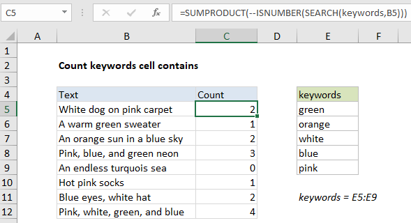
In the example shown, the formula in C5 is:

=SUMPRODUCT(--ISNUMBER(SEARCH(keywords,B5)))

where “keywords” is the named range E5:E9.

How this formula works

The core of this formula is the ISNUMBER + SEARCH approach to finding text in a cell, which is explained in more detail here. In this case, we are looking in each cell for all words in the named range “keywords” (E5:E9). We do this by passing the range into SEARCH as the find_text argument. Because we pass in an array of 5 items:

{"green";"orange";"white";"blue";"pink"}

we get an array of 5 items back as a result:

{#VALUE!;#VALUE!;1;#VALUE!;14}

Numbers correspond to matches, and the #VALUE! error means no match was found. In this case, because we don’t care where the text was found in the cell, we use ISNUMBER to convert the array into TRUE and FALSE values:

{FALSE;FALSE;TRUE;FALSE;TRUE}

And the double negative (–) to change these into 1s and zeros:

{0;0;1;0;1}

The SUMPRODUCT function then simply returns the sum of the array, 2 in this case.

Handling empty keywords

If the keyword range contains empty cells, the formula won’t work correctly, because the SEARCH function returns zero when looking for an empty string (“”). To filter any empty cells in the keyword range, you can use the variation below:

{=SUMPRODUCT(--ISNUMBER(SEARCH(IF(keywords<>"",keywords),B5)))}

Post navigation

Previous Post:

DECIMAL function: Description, Usage, Syntax, Examples and Explanation

Next Post:

AVERAGE function: Description, Usage, Syntax, Examples and Explanation

Leave a Reply Cancel reply

Your email address will not be published. Required fields are marked *

Learn Basic Excel

Ribbon
Workbook
Worksheets
Format Cells
Find & Select
Sort & Filter
Templates
Print
Share
Protect
Keyboard Shortcuts

Categories

  • Charts
  • Data Analysis
  • Data Validation
  • Excel Functions
    • Cube Functions
    • Database Functions
    • Date and Time Functions
    • Engineering Functions
    • Financial Functions
    • Information Functions
    • Logical Functions
    • Lookup and Reference Functions
    • Math and Trig Functions
    • Statistical Functions
    • Text Functions
    • Web Functions
  • Excel VBA
  • Excel Video Tutorials
  • Formatting
  • Grouping
  • Others

Logical Functions

  • SWITCH function: Description, Usage, Syntax, Examples and Explanation
  • Extract multiple matches into separate rows in Excel
  • TRUE function: Description, Usage, Syntax, Examples and Explanation
  • IFERROR function: Description, Usage, Syntax, Examples and Explanation
  • FALSE function: Description, Usage, Syntax, Examples and Explanation

Date Time

  • Calculate number of hours between two times in Excel
  • Calculate days remaining in Excel
  • Convert Excel time to decimal seconds
  • Display the current date and time in Excel
  • WORKDAY.INTL function: Description, Usage, Syntax, Examples and Explanation

Grouping

  • How to randomly assign data to groups in Excel
  • Group times into unequal buckets in Excel
  • Group numbers at uneven intervals in Excel
  • Running count group by n size in Excel
  • Calculate conditional mode with criteria in Excel

General

  • Convert column number to letter in Excel
  • How to calculate profit margin percentage in Excel
  • Count cells that contain errors in Excel
  • Convert column letter to number in Excel
  • AutoFit Column Width, AutoFit Row Height in Excel
© 2025 xlsoffice . All Right Reserved. | Teal Smiles | Abbreviations And Their Meaning