Find most frequent text within a range with criteria in Excel

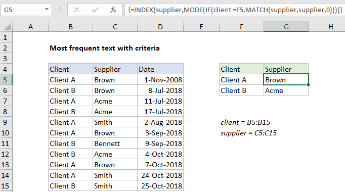
In the example shown, the formula in G5 is:

=INDEX(supplier,MODE(IF(client=F5,
MATCH(supplier,supplier,0))))

where “supplier” is the named range B5:B15, and “client” is the named range C5:C15.

How this formula works

Working from the inside out, we use the MATCH function to match the text range against itself, by giving MATCH the same range for lookup value and lookup array, with zero for match type:

MATCH(supplier,supplier,0)

Since the lookup value is an array with 10 values, MATCH returns an array of 10 results:

{1;1;3;3;5;1;7;3;1;5;5}

Each item in this array represents the first position at which a supplier name appears in the data. This array is fed into the IF function, which is used to filter results for Client A only:

IF(client=F5,{1;1;3;3;5;1;7;3;1;5;5})

IF returns the filtered array to the MODE function:

{1;FALSE;3;FALSE;5;1;FALSE;FALSE;1;5;FALSE}

Notice only positions associated with Client A remain in the array. MODE ignores FALSE values and returns the most frequently occurring number to INDEX as the row number:

=INDEX(supplier,1)

Finally, with the named range “supplier” as the array, INDEX returns “Brown”, the most frequently occurring supplier for Client A.