Break ties with helper column and COUNTIF in Excel

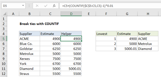
To break ties, you can use a helper column and the COUNTIF function to adjust values so that they don’t contain duplicates, and therefore won’t result in ties. In the example shown, the formula in D5 is:

=C5+(COUNTIF($C$5:C5,C5)-1)*0.01

Context

Sometimes, when you use functions like SMALL, LARGE, or RANK to rank highest or lowest values, you end up with ties, because the data contains duplicates. One way to break ties like this is to add a helper column with values that have been adjusted, then rank those values instead of the originals.

In this example, the logic used to adjust values is random – the first duplicate value will “win”, but you can adjust the formula to use logic that fits your particular situation and use case.

How this formula works

At the core, this formula uses the COUNTIF function and an expanding range to count occurrences of values. The expanding reference is used so that COUNTIFS returns a running count of occurrences, instead of a total count for each value:

COUNTIF($C$5:C5,C5)

Next, 1 is subtracted from the result (which makes the count of all non-duplicate values zero) and the result is multiplied by 0.01. This value is the “adjustment”, and intentionally small so as not to materially impact the original value.

In the example shown, Metrolux and Diamond both have the same estimate of $5000. Since Metrolux appears first in the list, the running count of 5000 is 1 and is cancelled out by subtracting 1, so the estimate is remains unchanged in the helper column:

=C8+(COUNTIF($C$5:C8,C8)-1)*0.01
=C8+(1-1)*0.01
=C8+0
=C8

However, for Diamond, the running count of 5000 is 2, so the estimate is adjusted:

=C11+(COUNTIF($C$5:C11,C11)-1)*0.01
=C11+(2-1)*0.01
=C11+1*0.01
=C11+0.01

Finally, the adjusted values are used for ranking instead of the original values in columns G and H.  The formula in G5 is:

=SMALL($D$5:$D$12,F5)

The formula in H5:

=INDEX($B$5:$B$12,MATCH(G5,$D$5:$D$12,0))