Skip to content
xlsoffice. All Rights Reserved
  • Home
  • Excel For Beginners
  • Excel Intermediate
  • Advanced Excel For Experts

Lookup and Reference Examples

  • How to get last column number in range in Excel
  • How to reference named range different sheet in Excel
  • Get nth match with INDEX / MATCH in Excel
  • Find Closest Match in Excel Using INDEX, MATCH, ABS and MIN functions
  • Extract all partial matches in Excel

Data Analysis Examples

  • Data Series in Excel
  • How to create Gauge Chart in Excel
  • How To Filter Data in Excel
  • How To Compare Two Lists in Excel
  • Everything about Charts in Excel

Data Validation Examples

  • How To Create Drop-down List in Excel
  • Excel Data validation whole percentage only
  • Excel Data validation no punctuation
  • Excel Data validation number multiple 100
  • Excel Data validation with conditional list

Count visible rows in a filtered list in Excel

by

This tutorial shows how to Count visible rows in a filtered list in Excel using the example below;

Formula

=SUBTOTAL(3,range)

Explanation

If you want to count the number of visible items in a filtered list, you can use the SUBTOTAL function, which automatically ignores rows that are hidden by a filter.

Worked Example:   Subtotal by invoice number in Excel

The SUBTOTAL function can perform calculations like COUNT, SUM, MAX, MIN, and more. (For a full list, see the table here). What makes SUBTOTAL especially interesting and useful is that it automatically ignores items that are not visible in a filtered list or table. This makes it ideal for showing how many items are visible in a list, the subtotal of visible rows, etc.

Worked Example:   Subtotal function in Excel

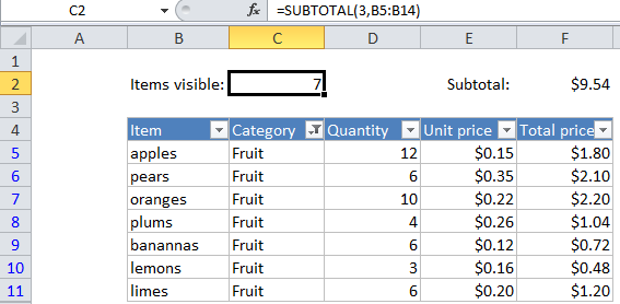
Following the example in the image above, to count the number of non-blank rows visible when a filter is active, use:

=SUBTOTAL(3,B5:B14)

If you are hiding rows manually (i.e. right-click, Hide), and not using the auto-filter, use this version instead:

=SUBTOTAL(103,B5:B14))

Post navigation

Previous Post:

Count paired items in listed combinations in Excel

Next Post:

Count unique values in a range with COUNTIF in Excel

Leave a Reply Cancel reply

Your email address will not be published. Required fields are marked *

Learn Basic Excel

Ribbon
Workbook
Worksheets
Format Cells
Find & Select
Sort & Filter
Templates
Print
Share
Protect
Keyboard Shortcuts

Categories

  • Charts
  • Data Analysis
  • Data Validation
  • Excel Functions
    • Cube Functions
    • Database Functions
    • Date and Time Functions
    • Engineering Functions
    • Financial Functions
    • Information Functions
    • Logical Functions
    • Lookup and Reference Functions
    • Math and Trig Functions
    • Statistical Functions
    • Text Functions
    • Web Functions
  • Excel VBA
  • Excel Video Tutorials
  • Formatting
  • Grouping
  • Others
  • How to split text string at specific character in Excel
  • Get last name from name with comma — Manipulating NAMES in Excel
  • How to pad text to match equal length in Excel
  • How to get first word in Excel
  • Join first and last name — Manipulating NAMES in Excel
  • Display Date is workday in Excel
  • How to calculate nth day of week in month in Excel
  • Calculate days remaining in Excel
  • ISOWEEKNUM function: Description, Usage, Syntax, Examples and Explanation
  • YEAR function: Description, Usage, Syntax, Examples and Explanation
  • PMT, RATE, NPER, PV and FV Financial Functions in Excel
  • Calculate payment periods for loan in Excel
  • PRICEMAT function: Description, Usage, Syntax, Examples and Explanation
  • TBILLPRICE function: Description, Usage, Syntax, Examples and Explanation
  • AMORDEGRC function: Description, Usage, Syntax, Examples and Explanation
© 2022 xlsoffice . All Right Reserved. | Teal Smiles