Skip to content
Free Excel Tutorials
  • Home
  • Excel For Beginners
  • Excel Intermediate
  • Advanced Excel For Experts

Data Analysis

  • How to conditionally sum numeric data in an Excel table using SUMIFS
  • How To Filter Data in Excel
  • How to Sort by Color in Excel
  • Number and Text Filters Examples in Excel
  • How to do a t-Test in Excel?

References

  • How to get last row in numeric data in Excel
  • Excel Advanced Lookup using Index and Match Functions
  • How to use Excel ROWS Function
  • Create hyperlink with VLOOKUP in Excel
  • Vlookup Examples in Excel

Data Validations

  • Excel Data validation no punctuation
  • How To Create Drop-down List in Excel
  • Excel Data validation must begin with
  • Data validation must not exist in list
  • Excel Data validation allow uppercase only

Excel Data validation number multiple 100

by

Accept only numbers that are multiple of 100

To allow only numbers in multiples of 100, you can use data validation with a custom formula based on the MOD function.

Formula

=MOD(A1,100)=0

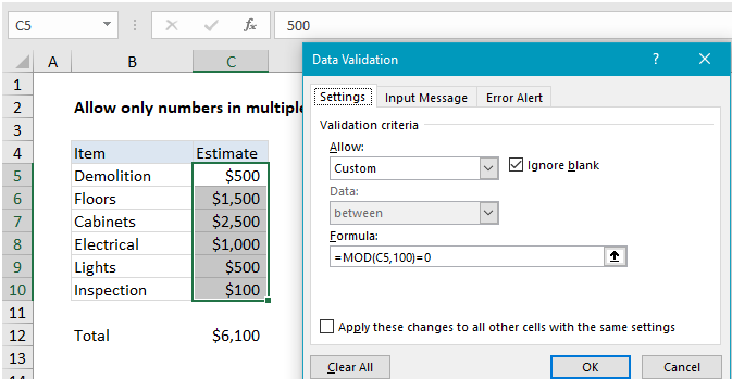
Note: Cell references in data validation formulas are relative to the upper left cell in the range selected when the validation rule is defined, in this case C5.

Explanation

In the example shown, the data validation applied to C5:C10 is:

=MOD(C5,100)=0

How this formula works

Data validation rules are triggered when a user adds or changes a cell value. When a custom formula returns TRUE, validation passes and the input is accepted. When the formula returns FALSE, validation fails and the input is rejected.

In this case, the MOD function is used to perform a modulo operation, which returns the remainder after division. The formula used to validate input is:

=MOD(C5,100)=0

The value in C5 is 500. The MOD function divides 500 by 100 and gets 5, with a remainder of zero. Since 0 = 0,  The rule returns TRUE and the data validation passes:

=MOD(500,100)=0
=0=0
=TRUE

If a user enters, say, 550, the remainder is 50, and validation fails:

=MOD(C5,100)=0
=MOD(550,100)=0
=50=0
=FALSE

Post navigation

Previous Post:

COSH function: Description, Usage, Syntax, Examples and Explanation

Next Post:

Excel Data validation require unique number

Leave a Reply Cancel reply

Your email address will not be published. Required fields are marked *

Learn Basic Excel

Ribbon
Workbook
Worksheets
Format Cells
Find & Select
Sort & Filter
Templates
Print
Share
Protect
Keyboard Shortcuts

Categories

  • Charts
  • Data Analysis
  • Data Validation
  • Excel Functions
    • Cube Functions
    • Database Functions
    • Date and Time Functions
    • Engineering Functions
    • Financial Functions
    • Information Functions
    • Logical Functions
    • Lookup and Reference Functions
    • Math and Trig Functions
    • Statistical Functions
    • Text Functions
    • Web Functions
  • Excel VBA
  • Excel Video Tutorials
  • Formatting
  • Grouping
  • Others

Logical Functions

  • XOR function: Description, Usage, Syntax, Examples and Explanation
  • How to use Excel OR Function
  • IFNA function: Description, Usage, Syntax, Examples and Explanation
  • IF with boolean logic in Excel
  • OR function: Description, Usage, Syntax, Examples and Explanation

Date Time

  • Calculate retirement date in Excel
  • Two ways to sum time over 30 minutes in Excel
  • Get days before a date in Excel
  • How to calculate next day of week in Excel
  • Series of dates by day

Grouping

  • Categorize text with keywords in Excel
  • Calculate conditional mode with criteria in Excel
  • Group numbers with VLOOKUP in Excel
  • Map inputs to arbitrary values in Excel
  • If cell contains one of many things in Excel

General

  • Share Excel data with Word documents
  • How to generate random times at specific intervals in Excel
  • Cell References: Relative, Absolute and Mixed Referencing Examples
  • Customize Ribbon In Excel
  • How to calculate percent change in Excel
© 2026 xlsoffice . All Right Reserved. | Teal Smiles | Abbreviations And Their Meaning