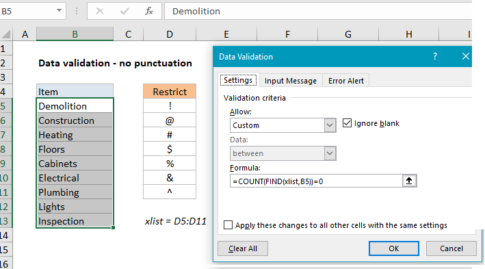
In the example shown, the data validation applied to C5:C10 is:

=COUNT(FIND(xlist,B5))=0

where xlist is the named range D5:D11.

How this formula works

Data validation rules are triggered when a user adds or changes a cell value. When a custom formula returns TRUE, validation passes and the input is accepted. When a formula returns FALSE, validation fails and the input is rejected with a popup message.

In this case, we have previous defined the named range “xlist” as D5:D11. This range holds characters that are not allowed.

The formula we are using for data validation is:

=COUNT(FIND(xlist,B5))=0

Working from the inside out FIND function is configured with xlist for “find text”, and cell B5 as the text to search. Because we are giving FIND an array with multiple values, FIND returns an array of result, one for each character in the named range “xlist”. For cell B5, the result from FIND looks like this:

{#VALUE!;#VALUE!;#VALUE!;#VALUE!;#VALUE!;#VALUE!;#VALUE!}

Each #VALUE error represents one character not found. If we try to enter, say, “demolition@”, which includes a restricted character, FIND returns:

{#VALUE!;11;#VALUE!;#VALUE!;#VALUE!;#VALUE!;#VALUE!}

Note the second value in the array is now 11.

Next, the COUNT function returns the count of all numbers in the array. When the array contains no numbers (i.e. no restricted characters) COUNT returns zero, the expression returns TRUE, and data validation succeeds. However, When the array contains no numbers (i.e. there is at least one restricted character found) COUNT returns a number, the expression returns FALSE, and data validation fails.