Understanding Pivot Tables in Excel

Pivot tables are one of Excel’s most powerful features. A pivot table allows you to extract the significance from a large, detailed data set.

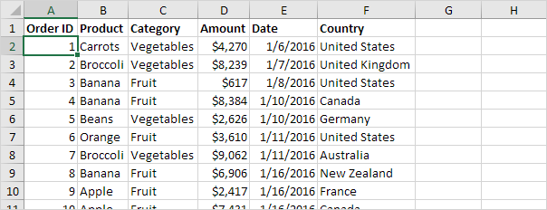
Our data set consists of 213 records and 6 fields. Order ID, Product, Category, Amount, Date and Country.

Insert a Pivot Table

To insert a pivot table, execute the following steps.

1. Click any single cell inside the data set.

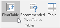
2. On the Insert tab, in the Tables group, click PivotTable.

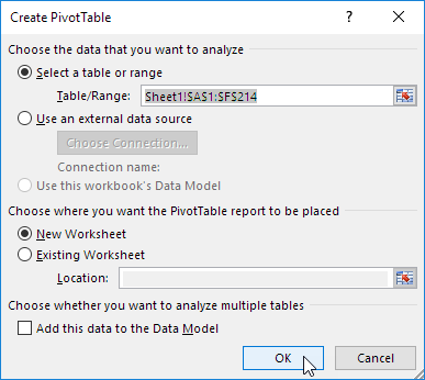
The following dialog box appears. Excel automatically selects the data for you. The default location for a new pivot table is New Worksheet.

3. Click OK.

Drag fields

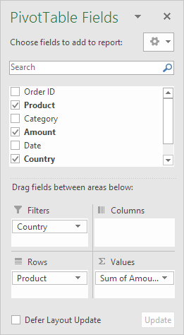
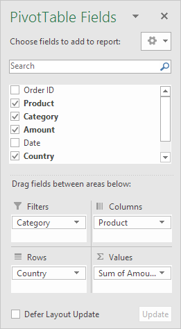
The PivotTable Fields pane appears. To get the total amount exported of each product, drag the following fields to the different areas.

1. Product field to the Rows area.

2. Amount field to the Values area.

3. Country field to the Filters area.

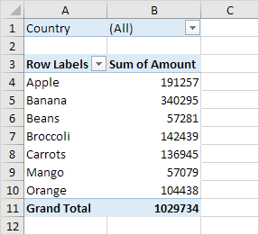
Below you can find the pivot table. Bananas are our main export product. That’s how easy pivot tables can be!

Sort

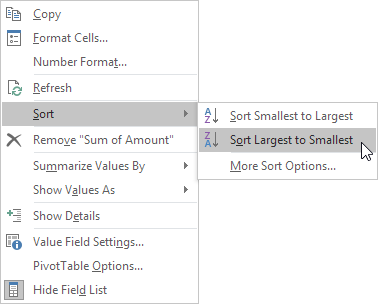
To get Banana at the top of the list, sort the pivot table.

1. Click any cell inside the Sum of Amount column.

2. Right click and click on Sort, Sort Largest to Smallest.

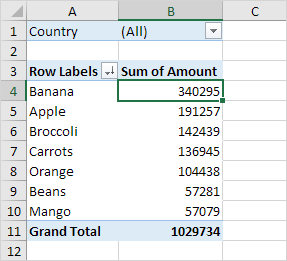
Result.

Filter

Because we added the Country field to the Filters area, we can filter this pivot table by Country. For example, which products do we export the most to France?

1. Click the filter drop-down and select France.

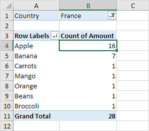
Result. Apples are our main export product to France.

Note: you can use the standard filter (triangle next to Row Labels) to only show the amounts of specific products.

Change Summary Calculation

By default, Excel summarizes your data by either summing or counting the items. To change the type of calculation that you want to use, execute the following steps.

1. Click any cell inside the Sum of Amount column.

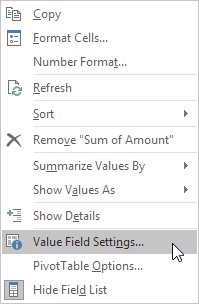
2. Right click and click on Value Field Settings.

3. Choose the type of calculation you want to use. For example, click Count.

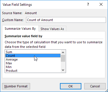
4. Click OK.

Result. 16 out of the 28 orders to France were ‘Apple’ orders.

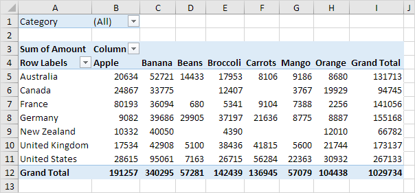
Two-dimensional Pivot Table

If you drag a field to the Rows area and Columns area, you can create a two-dimensional pivot table. First, insert a pivot table. Next, to get the total amount exported to each country, of each product, drag the following fields to the different areas.

1. Country field to the Rows area.

2. Product field to the Columns area.

3. Amount field to the Values area.

4. Category field to the Filters area.

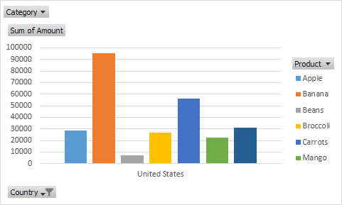
Below you can find the two-dimensional pivot table.

To easily compare these numbers, create a pivot chart and apply a filter. Maybe this is one step too far for you at this stage, but it shows you one of the many other powerful pivot table features Excel has to offer.