How to create dynamic reference table name in Excel

To build a formula with a dynamic reference to an Excel Table name, you can use the INDIRECT function with concatenation as needed.

Formula

=SUM(INDIRECT(table&"[column]"))

Note: INDIRECT is a volatile function and can cause performance issues in larger, more complex workbooks.

Explanation

In the example shown, the formula in L5 is:

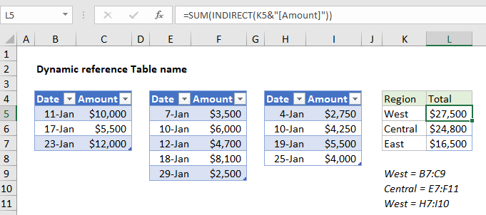
=SUM(INDIRECT(K5&"[Amount]"))

Which returns the SUM of Amounts for three tables named “West”, “Central”, and “East”.

How this formula works

This formula behaves like these simpler formulas:

=SUM(West[Amount])
=SUM(Central[Amount])
=SUM(East[Amount])

However, instead of hardcoding the table into each SUM formula, the table names are listed in column K, and the formulas in column L use concatenation to assemble a reference to each table. This allows the same formula to be used in L5:L7.

The trick is the INDIRECT function to evaluate the reference.

We start with:

=SUM(INDIRECT(K5&"[Amount]"))

which becomes:

=SUM(INDIRECT("West"&"[Amount]"))

and then:

=SUM(INDIRECT("West[Amount]"))

The INDIRECT function then resolves the text string into a proper structured reference:

=SUM(West[Amount])

And the SUM function returns the final result, 27,500 for the West region.