Skip to content
Free Excel Tutorials
  • Home
  • Excel For Beginners
  • Excel Intermediate
  • Advanced Excel For Experts

Data Analysis

  • Create Scatter Chart in Excel
  • Conditional Formatting Data bars Examples in Excel
  • How To Create Pareto Chart in Excel
  • Understanding Anova in Excel
  • How To Remove Duplicates In Excel Column Or Row?

References

  • To count total rows in a range in Excel
  • Basic INDEX MATCH approximate in Excel
  • Extract all partial matches in Excel
  • How to use Excel ROW Function
  • How to get first column number in range in Excel

Data Validations

  • Excel Data validation don’t exceed total
  • Excel Data validation must begin with
  • Excel Data validation must contain specific text
  • Excel Data validation exists in list
  • Excel Data validation date in next 30 days

How to create dynamic reference table name in Excel

by

To build a formula with a dynamic reference to an Excel Table name, you can use the INDIRECT function with concatenation as needed.

Formula

=SUM(INDIRECT(table&"[column]"))
Note: INDIRECT is a volatile function and can cause performance issues in larger, more complex workbooks.

Explanation

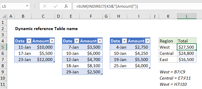
In the example shown, the formula in L5 is:

=SUM(INDIRECT(K5&"[Amount]"))

Which returns the SUM of Amounts for three tables named “West”, “Central”, and “East”.

How this formula works

This formula behaves like these simpler formulas:

=SUM(West[Amount])
=SUM(Central[Amount])
=SUM(East[Amount])

However, instead of hardcoding the table into each SUM formula, the table names are listed in column K, and the formulas in column L use concatenation to assemble a reference to each table. This allows the same formula to be used in L5:L7.

The trick is the INDIRECT function to evaluate the reference.

We start with:

=SUM(INDIRECT(K5&"[Amount]"))

which becomes:

=SUM(INDIRECT("West"&"[Amount]"))

and then:

=SUM(INDIRECT("West[Amount]"))

The INDIRECT function then resolves the text string into a proper structured reference:

=SUM(West[Amount])

And the SUM function returns the final result, 27,500 for the West region.

Post navigation

Previous Post:

How to calculate project complete percentage in Excel

Next Post:

Popularly Used Excel Functions and their examples

Leave a Reply Cancel reply

Your email address will not be published. Required fields are marked *

Learn Basic Excel

Ribbon
Workbook
Worksheets
Format Cells
Find & Select
Sort & Filter
Templates
Print
Share
Protect
Keyboard Shortcuts

Categories

  • Charts
  • Data Analysis
  • Data Validation
  • Excel Functions
    • Cube Functions
    • Database Functions
    • Date and Time Functions
    • Engineering Functions
    • Financial Functions
    • Information Functions
    • Logical Functions
    • Lookup and Reference Functions
    • Math and Trig Functions
    • Statistical Functions
    • Text Functions
    • Web Functions
  • Excel VBA
  • Excel Video Tutorials
  • Formatting
  • Grouping
  • Others

Logical Functions

  • How to use Excel XOR Function
  • Excel If, Nested If, And/Or Criteria Examples
  • Nested IF function example in Excel
  • OR function: Description, Usage, Syntax, Examples and Explanation
  • IF, AND, OR and NOT Functions Examples in Excel

Date Time

  • How to calculate most recent day of week in Excel
  • Convert Excel time to decimal hours in Excel
  • DAYS function: Description, Usage, Syntax, Examples and Explanation
  • Count holidays between two dates in Excel
  • Get fiscal quarter from date in Excel

Grouping

  • Group times into 3 hour buckets in Excel
  • Running count group by n size in Excel
  • Categorize text with keywords in Excel
  • Map text to numbers in Excel
  • If cell contains one of many things in Excel

General

  • Split Cell Content Using Text to Columns in Excel
  • Currency vs Accounting Format in Excel
  • Create dynamic workbook reference to another workbook in Excel
  • Zoom Worksheet in Excel
  • Basic text sort formula in Excel
© 2025 xlsoffice . All Right Reserved. | Teal Smiles | Abbreviations And Their Meaning