Skip to content
Free Excel Tutorials
  • Home
  • Excel For Beginners
  • Excel Intermediate
  • Advanced Excel For Experts

Data Analysis

  • Managing Conditional Formatting Rules in Excel
  • How To Perform and Interpret Regression Analysis in Excel
  • How to calculate average last N values in a table in Excel
  • Excel Line Chart
  • How to create dynamic reference table name in Excel

References

  • How to calculate two-way lookup VLOOKUP in Excel Table
  • Perform case-sensitive Lookup in Excel
  • Merge tables with VLOOKUP in Excel
  • VLOOKUP function: Description, Usage, Syntax, Examples and Explanation
  • How to use Excel LOOKUP Function

Data Validations

  • Excel Data validation unique values only
  • Excel Data validation allow uppercase only
  • Excel Data validation require unique number
  • Excel Data validation must not contain
  • Data validation must not exist in list

How to get relative column numbers in a range in Excel

by

This tutorial shows how to get a full set of relative column numbers in a range using an array formula based on the COLUMN function.

Formula

{=COLUMN(range)-COLUMN(range.firstcell)+1}


On the worksheet, this must be entered as multi-cell array formula using Control + Shift + Enter

This is a robust formula that will continue to generate relative numbers even when columns are inserted in front of the range.

Explanation

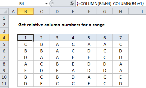
In the example shown, the array formula in B4:H4 is:

{=COLUMN(B4:H4)-COLUMN(B4)+1}

How this formula works

The first COLUMN function generates an array of 7 numbers like this:

{2,3,4,5,6,7,8}

The second COLUMN function generates an array with just one item like this:

{2}

which is then subtracted from the first array to yield:

{0,1,2,3,4,5,6}

Finally, 1 is added to get:

{1,2,3,4,5,6,7}

With a named range

You can adapt this formula to use with a named range. For example, in the above example, if you created a named range “data” for B4:H4, you can use this formula to generate column numbers:

{=COLUMN(data)-COLUMN(INDEX(data,1,1))+1}

Post navigation

Previous Post:

How to calculate project complete percentage in Excel

Next Post:

Popularly Used Excel Functions and their examples

Leave a Reply Cancel reply

Your email address will not be published. Required fields are marked *

Learn Basic Excel

Ribbon
Workbook
Worksheets
Format Cells
Find & Select
Sort & Filter
Templates
Print
Share
Protect
Keyboard Shortcuts

Categories

  • Charts
  • Data Analysis
  • Data Validation
  • Excel Functions
    • Cube Functions
    • Database Functions
    • Date and Time Functions
    • Engineering Functions
    • Financial Functions
    • Information Functions
    • Logical Functions
    • Lookup and Reference Functions
    • Math and Trig Functions
    • Statistical Functions
    • Text Functions
    • Web Functions
  • Excel VBA
  • Excel Video Tutorials
  • Formatting
  • Grouping
  • Others

Logical Functions

  • SWITCH function example in Excel
  • How to use Excel AND Function
  • IF with boolean logic in Excel
  • Invoice status with nested if in Excel
  • TRUE function: Description, Usage, Syntax, Examples and Explanation

Date Time

  • WORKDAY.INTL function: Description, Usage, Syntax, Examples and Explanation
  • Get days before a date in Excel
  • DATEDIF function: Description, Usage, Syntax, Examples and Explanation
  • Count holidays between two dates in Excel
  • EDATE function: Description, Usage, Syntax, Examples and Explanation

Grouping

  • Group arbitrary text values in Excel
  • Running count group by n size in Excel
  • Group numbers at uneven intervals in Excel
  • Map inputs to arbitrary values in Excel
  • Group times into unequal buckets in Excel

General

  • Automatically fill series of cells in Excel using AutoFill
  • How to get Excel workbook path only
  • Zoom Worksheet in Excel
  • List sheet names with formula in Excel
  • Select, Insert, Rename, Move, Delete Worksheets in Excel
© 2025 xlsoffice . All Right Reserved. | Teal Smiles | Abbreviations And Their Meaning