Calculate cumulative loan interest in Excel

To calculate the cumulative principal paid between any two loan payments, you can use the CUMIPMT function. In the example shown, we calculate the total principal paid over the full term of the loan by using the first and last period.

Formula

=CUMIPMT(rate,nper,pv,start,end,type)

Explanation

The formula in C10 is:

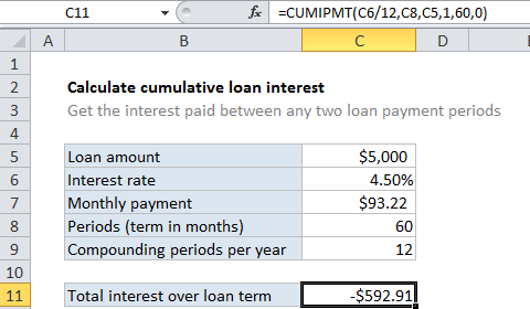
=CUMIPMT(C6/12,C8,C5,1,60,0)

How this formula works

For this example, we want to calculate cumulative interest over the full term of a 5-year loan of $5,000 with an interest rate of 4.5%. To do this, we set up CUMIPMT like this:

rate – The interest rate per period. We divide the value in C6 by 12 since 4.5% represents annual interest:

=C6/12

nper – the total number of payment periods for the loan, 60, from cell C8.

pv – The present value, or total value of all payments now, 5000, from cell C5.

start_period – the first period of interest, 1 in this case, since we are calculating principal across the entire loan term.

end_period – the last period of interest, 60 in this case for the full loan term.

With these inputs, the CUMIPMT function returns -592.91, the total interest paid for the loan.